

barbac is an R package for end-to-end DNA barcode
lineage tracking. This vignette walks through the core R-level workflow
— clustering a count table with super_cluster2() and
visualising a time series with barbac_ts_area() — without
requiring any external CLI tools. For the full FASTQ→BAM pipeline
(FastQC → PEAR → minimap2 → samtools), see
?run_cli_pipeline.
A tiny synthetic dataset
We build a toy dataset of 4 true barcodes, each seeded from a 20-nucleotide random sequence, with 100 noisy reads per barcode. Each read has a per-base substitution probability of 1%.
alphabet <- c("A", "C", "G", "T")

random_barcode <- function(len = 20) {
  paste0(sample(alphabet, len, replace = TRUE), collapse = "")
}

mutate_seq <- function(seq, sub_rate = 0.01) {
  bases <- strsplit(seq, "")[[1]]
  hit   <- runif(length(bases)) < sub_rate
  bases[hit] <- vapply(bases[hit], function(b) {
    sample(setdiff(alphabet, b), 1L)
  }, character(1))
  paste0(bases, collapse = "")
}

true_barcodes <- vapply(1:4, function(i) random_barcode(), character(1))
true_barcodes
#> [1] "ATGACAGGCCGGAAACCCCG" "AGAAAACAACCCATGATGCC" "CCGTTTCTAGCATTAGTCCG"
#> [4] "GCCTTCCACCCCAGGTCGGT"

reads <- unlist(lapply(true_barcodes, function(b) {
  replicate(100, mutate_seq(b, sub_rate = 0.01))
}))

# Collapse to unique-sequence counts
input <- as.data.frame(table(reads), stringsAsFactors = FALSE)
names(input) <- c("barcode", "counts")
input <- input[order(-input$counts), ]
head(input)
#>                 barcode counts
#> 49 CCGTTTCTAGCATTAGTCCG     81
#> 5  AGAAAACAACCCATGATGCC     80
#> 21 ATGACAGGCCGGAAACCCCG     78
#> 61 GCCTTCCACCCCAGGTCGGT     77
#> 19 ATAACAGGCCGGAAACCCCG      3
#> 43 CCGTTTCAAGCATTAGTCCG      3
Clustering with super_cluster2()
super_cluster2() accepts either a data.frame with
columns barcode and counts, or a path to a CSV
in the same layout. Here we pass the data.frame directly and use a
Levenshtein distance threshold of 2.
result <- super_cluster2(
  input,
  distance    = 2,
  merge_ratio = 20,
  verbose     = FALSE
)
result
#> # A tibble: 4 × 5
#>   cluster_id central_barcode      all_barcodes all_counts sum_counts
#>   <chr>      <chr>                <list>       <list>          <int>
#> 1 group1     CCGTTTCTAGCATTAGTCCG <chr [18]>   <int [18]>        100
#> 2 group2     AGAAAACAACCCATGATGCC <chr [18]>   <int [18]>        100
#> 3 group3     ATGACAGGCCGGAAACCCCG <chr [18]>   <int [18]>        100
#> 4 group4     GCCTTCCACCCCAGGTCGGT <chr [22]>   <int [22]>        100
Each row is one cluster: central_barcode is the
abundance-ranked representative, all_barcodes and
all_counts are the member barcodes and their raw counts,
and sum_counts is the summed abundance.
We can check how well the clustering recovered the true barcodes:
Visualising a time series
barbac_ts_area() takes a table of counts across
timepoints and returns a stacked-area ggplot of per-timepoint
frequencies. It accepts long-format input directly:
tp   <- 0:20                                            # 21 timepoints
n_tp <- length(tp)

ts_long <- dplyr::bind_rows(
  tibble(barcode = "A", time = tp,
         counts = round(seq(1000, 200, length.out = n_tp))),    # falling
  tibble(barcode = "B", time = tp,
         counts = round(seq( 200, 1000, length.out = n_tp))),   # rising
  tibble(barcode = "C", time = tp,
         counts = ifelse(tp < 8, 0,
                         round(seq(0, 800, length.out = n_tp - 7 + 1))[-1])), # late arrival
  tibble(barcode = "D", time = tp, counts = 50)                 # constant
)

barbac_ts_area(ts_long, min_total_count = 0)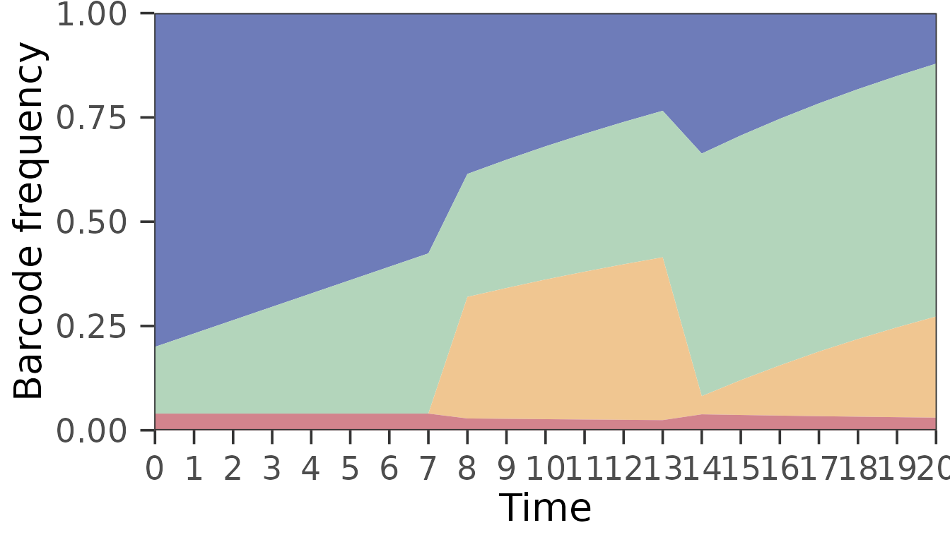
Lineage C illustrates the “late arrivals” case: it has zero counts at
timepoints 0–7, but is carried through the full series because
include_late = TRUE (the default) and missing cells are
filled with a small ε.
The same function auto-detects Bartender’s wide export layout:
set.seed(11)

ts_wide <- cbind(
  tibble(
    Cluster.ID    = sprintf("bc%02d", 1:5),
    Center        = c("ACGT", "ACGA", "ACCA", "TGGT", "GACC"),
    Cluster.Score = round(runif(5, 0.7, 1), 2)
  ),
  setNames(
    as.data.frame(matrix(rpois(5 * 20, 100), nrow = 5)),
    sprintf("time_point_%d", 1:20)
  )
)

barbac_ts_area(ts_wide, min_total_count = 0)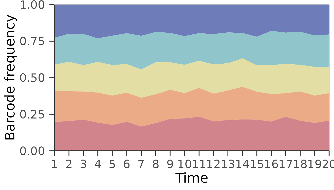
If the layout is neither long nor Bartender-wide, the function stops with a clear error that lists the expected column names.
Styling — theme_barbac() is applied by default
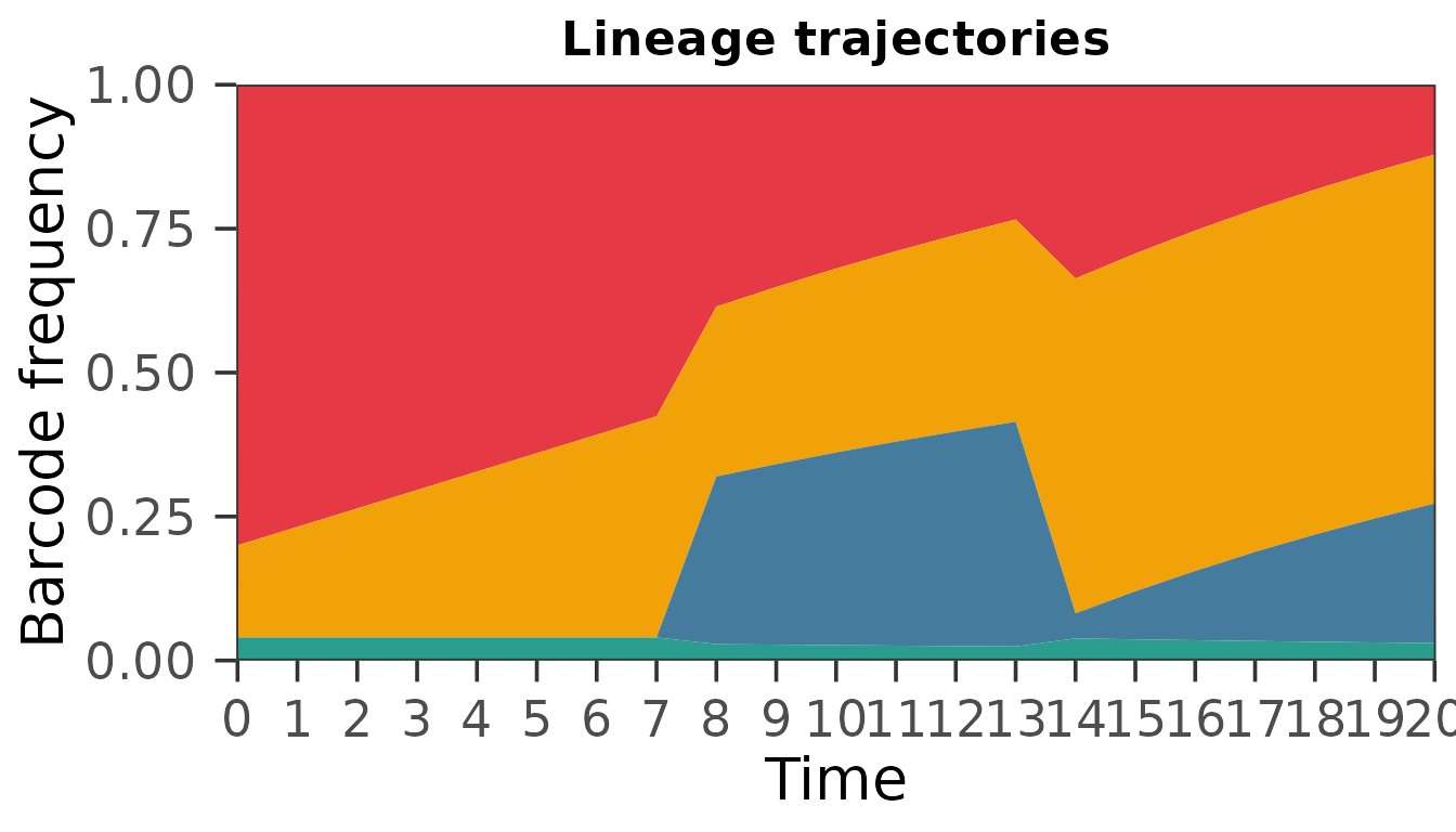
barbac_ts_area() returns a ggplot object
that has already been styled with the package’s publication-ready theme,
theme_barbac()
— minimal grid, visible ticks, solid inner border, centred bold title,
bottom legend. There is nothing to add: just call the function.
barbac_ts_area(
  ts_long,
  min_total_count = 0,
  palette         = c("#E63946", "#F1A208", "#457B9D", "#2A9D8F"),
  title           = "Lineage trajectories"
)
Pass theme = NULL to get a stock ggplot back, or
theme = ... to swap in any other theme (including
theme_barbac(base_size = 18, family = "Avenir") for
slide-friendly output).
# Bigger font + Avenir on macOS
barbac_ts_area(ts_long, min_total_count = 0,
               theme = theme_barbac(base_size = 18, family = "Avenir"))

# Unthemed - roll your own
barbac_ts_area(ts_long, min_total_count = 0, theme = NULL) +
  ggplot2::theme_classic()
Fonts
The theme’s family argument defaults to
"sans" so plots render on every platform without extra
setup. On macOS you already have Avenir installed. For a similar
geometric-sans look on Linux/Windows, register a Google Font at runtime
through showtext:
sysfonts::font_add_google("Nunito Sans", "nunito")
showtext::showtext_auto()
barbac_ts_area(ts_long, min_total_count = 0,
               theme = theme_barbac(family = "nunito"))
Avenir is a commercial Adobe font and cannot be redistributed inside
the package, so theme_barbac() never bundles a font — it
just points at whatever family you name.
Interactive plots
Set interactive = TRUE to get an interactive widget with
hover tooltips revealing the barcode identifier, timepoint and frequency
for whichever band the cursor is on. Two backends are supported:
-
interactive = TRUE(the default when interactivity is requested) or"ggiraph"uses ggiraph: preserves the exact ggplot look, snappy hover on stacked areas, lightweight SVG output. -
interactive = "plotly"uses plotly: built-in zoom / pan / lasso, but a slightly heavier bundle and minor theme drift.
barbac_ts_area(
  ts_long,
  min_total_count = 0,
  palette         = c("#E63946", "#F1A208", "#457B9D", "#2A9D8F"),
  interactive     = TRUE
)
The static and interactive paths accept exactly the same arguments;
only the return type differs (ggplot versus
girafe or plotly htmlwidget).
Multilineage
The four-lineage toy above demonstrates the API. In practice
barbac_ts_area() is designed to handle the many-lineage
output of a real barcode-sequencing experiment. Here we simulate a
100-lineage community across 21 timepoints, with log-normal initial
abundances and a small Gaussian fitness effect per lineage, and plot
every lineage using the minou palette from the ltc
package.
set.seed(7)

n_bar   <- 100
tp      <- 0:20                       # 21 timepoints
depth   <- 1e6

barcodes  <- sprintf("bc_%03d", seq_len(n_bar))
fitness   <- rnorm(n_bar, mean = 0, sd = 0.20)
init_freq <- rlnorm(n_bar, meanlog = 0, sdlog = 1.5)
init_freq <- init_freq / sum(init_freq)

ts_multi <- do.call(rbind, lapply(tp, function(t) {
  raw   <- init_freq * exp(fitness * t)
  freq  <- raw / sum(raw)
  tibble::tibble(
    barcode = barcodes,
    time    = t,
    counts  = round(freq * depth)
  )
}))

# One colour per barcode, interpolated from the minou seed palette
# (same pattern as the phage.colors helper in the ltc README).
phage_colors <- function(df) {
  n <- dplyr::n_distinct(df$barcode)
  pal <- if (requireNamespace("ltc", quietly = TRUE)) {
    ltc::ltc("minou", n, type = "continuous")
  } else {
    viridisLite::magma(n, begin = 0.05, end = 0.95)  # fallback
  }
  grDevices::colorRampPalette(pal)(n)
}

barbac_ts_area(
  ts_multi,
  min_total_count = 0,                            # plot every lineage
  palette         = phage_colors(ts_multi),
  title           = "Multilineage — 100 barcodes across 21 timepoints"
)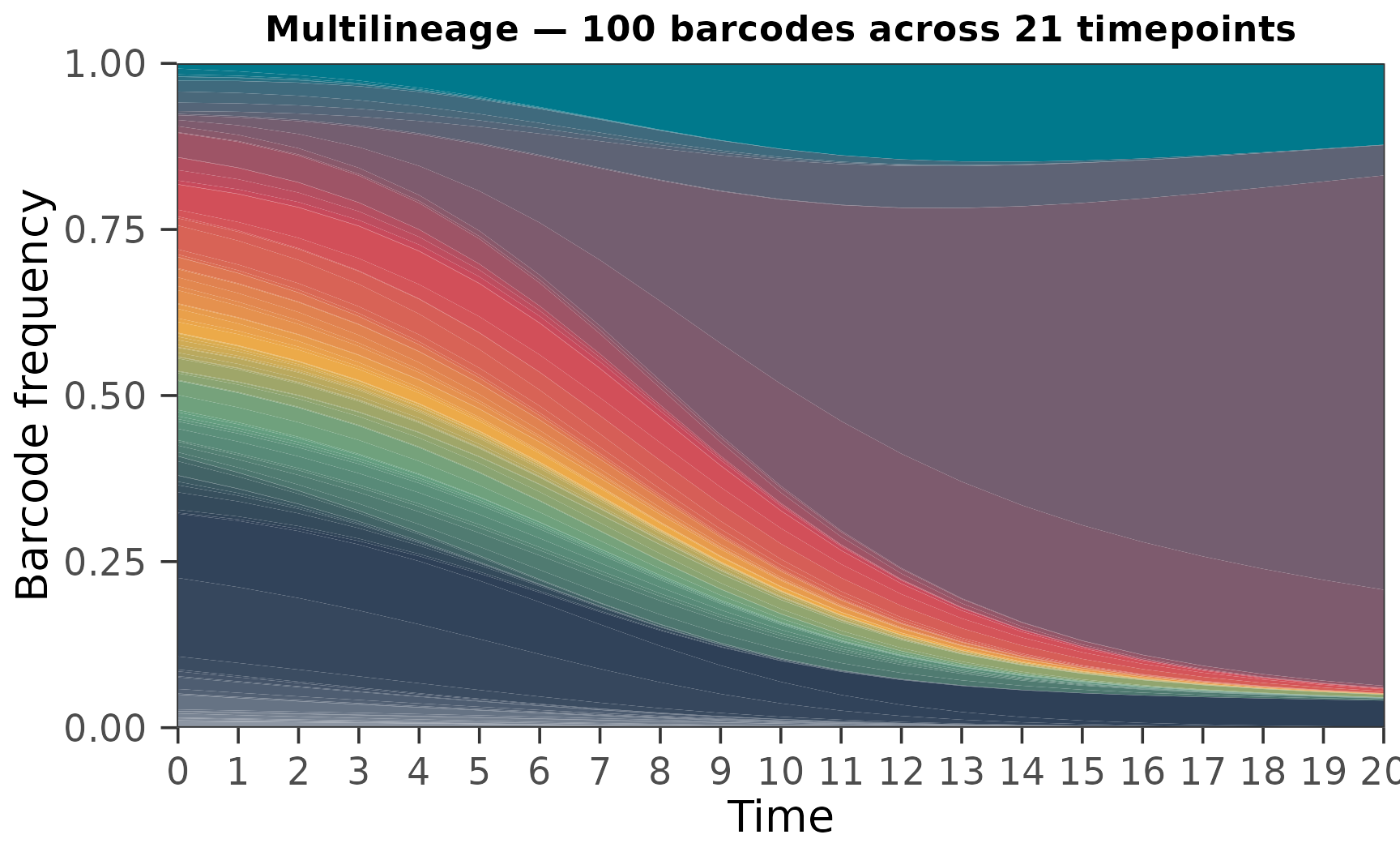
Every timepoint fills the stack to y = 1 exactly. Lineages with positive fitness sweep upward across the 21 timepoints; negative-fitness lineages shrink; neutral ones drift proportionally to their initial abundance.
The ltc package is available from GitHub via
remotes::install_github("loukesio/ltc_palettes"). Any
character vector of colour hex codes works as palette, so
viridisLite::magma(),
RColorBrewer::brewer.pal(), a manual palette, or any other
source are equally valid.
The same plot, interactively
At this diversity the static plot is useful for overall shape but
useless for identifying individual lineages. Setting
interactive = TRUE returns an interactive widget with
per-band hover tooltips showing the barcode identifier, timepoint and
frequency.
barbac_ts_area() supports two interactive backends:
-
interactive = TRUE(or"ggiraph", the default) — renders viaggiraph, which preserves the exact ggplot look, produces a lightweight SVG-based widget, and performs well with hundreds of stacked polygons. -
interactive = "plotly"— renders viaplotly’sggplotly(), which gives you built-in zoom / pan / lasso at the cost of a slightly drifted theme and a heavier HTML page.
barbac_ts_area(
  ts_multi,
  min_total_count = 0,
  palette         = phage_colors(ts_multi),
  title           = "Multilineage — hover over a band for its barcode",
  interactive     = TRUE                                # = "ggiraph"
)
If you prefer plotly’s zoom / pan controls:
barbac_ts_area(
  ts_multi,
  min_total_count = 0,
  palette         = phage_colors(ts_multi),
  title           = "Multilineage (plotly backend)",
  interactive     = "plotly"
)
What is super_cluster2() doing?
Briefly: the algorithm sorts input sequences by descending abundance,
scans each sequence for candidate centroids within edit distance
distance using a two-tier Hamming/Levenshtein index, scores
candidates with a count-aware log-likelihood, and either merges the
sequence into the best-scoring parent (subject to a distance-aware
count-ratio guard) or seeds a new cluster. A post-hoc refinement pass
promotes over-represented children of large clusters and reassigns their
neighbours.
On the Johnson et al. (2023) 100k-barcode benchmark
super_cluster2() matches Shepherd on the four Johnson
metrics (Pearson R, FN%, FP%, WS%) while running roughly 1.7× faster.
When indel errors are added to the simulator — which is where Shepherd’s
Hamming-based index struggles — super_cluster2()’s
wrong-sequence rate stays an order of magnitude below Shepherd’s.
Reproducibility scripts live in the benchmark/ directory of
the package repository.
Full FASTQ-to-lineage pipeline
For a complete analysis starting from raw FASTQ files,
barbac ships a CLI-wrapping pipeline that runs FastQC,
PEAR, minimap2 and samtools, then extracts barcodes at fixed genomic
coordinates and hands the result to super_cluster2(). See
?run_cli_pipeline, ?barbac_xtr and
?configure_environment for details.
Session info
sessionInfo()
#> R version 4.6.1 (2026-06-24)
#> Platform: x86_64-pc-linux-gnu
#> Running under: Ubuntu 24.04.4 LTS
#>
#> Matrix products: default
#> BLAS:   /usr/lib/x86_64-linux-gnu/openblas-pthread/libblas.so.3
#> LAPACK: /usr/lib/x86_64-linux-gnu/openblas-pthread/libopenblasp-r0.3.26.so;  LAPACK version 3.12.0
#>
#> locale:
#>  [1] LC_CTYPE=C.UTF-8       LC_NUMERIC=C           LC_TIME=C.UTF-8
#>  [4] LC_COLLATE=C.UTF-8     LC_MONETARY=C.UTF-8    LC_MESSAGES=C.UTF-8
#>  [7] LC_PAPER=C.UTF-8       LC_NAME=C              LC_ADDRESS=C
#> [10] LC_TELEPHONE=C         LC_MEASUREMENT=C.UTF-8 LC_IDENTIFICATION=C
#>
#> time zone: UTC
#> tzcode source: system (glibc)
#>
#> attached base packages:
#> [1] stats     graphics  grDevices utils     datasets  methods   base
#>
#> other attached packages:
#> [1] dplyr_1.2.1  tibble_3.3.1 barbac_0.1.0
#>
#> loaded via a namespace (and not attached):
#>  [1] ggiraph_0.9.6               tidyselect_1.2.1
#>  [3] farver_2.1.2                Biostrings_2.80.1
#>  [5] S7_0.2.2                    bitops_1.0-9
#>  [7] fastmap_1.2.0               tweenr_2.0.3
#>  [9] fontquiver_0.2.1            GenomicAlignments_1.48.0
#> [11] digest_0.6.39               lifecycle_1.0.5
#> [13] magrittr_2.0.5              compiler_4.6.1
#> [15] rlang_1.2.0                 sass_0.4.10
#> [17] tools_4.6.1                 utf8_1.2.6
#> [19] yaml_2.3.12                 knitr_1.51
#> [21] S4Arrays_1.12.0             labeling_0.4.3
#> [23] htmlwidgets_1.6.4           DelayedArray_0.38.2
#> [25] RColorBrewer_1.1-3          abind_1.4-8
#> [27] BiocParallel_1.46.0         withr_3.0.3
#> [29] purrr_1.2.2                 BiocGenerics_0.58.1
#> [31] desc_1.4.3                  grid_4.6.1
#> [33] polyclip_1.10-7             stats4_4.6.1
#> [35] gdtools_0.5.1               colorspace_2.1-2
#> [37] ggplot2_4.0.3               scales_1.4.0
#> [39] MASS_7.3-65                 SummarizedExperiment_1.42.0
#> [41] cli_3.6.6                   rmarkdown_2.31
#> [43] crayon_1.5.3                ragg_1.5.2
#> [45] generics_0.1.4              otel_0.2.0
#> [47] stringdist_0.9.17           tzdb_0.5.0
#> [49] cachem_1.1.0                ggforce_0.5.0
#> [51] stringr_1.6.0               PNWColors_0.1.0
#> [53] parallel_4.6.1              XVector_0.52.0
#> [55] matrixStats_1.5.0           vctrs_0.7.3
#> [57] Matrix_1.7-5                jsonlite_2.0.0
#> [59] fontBitstreamVera_0.1.1     IRanges_2.46.0
#> [61] hms_1.1.4                   patchwork_1.3.2
#> [63] S4Vectors_0.50.1            systemfonts_1.3.2
#> [65] jquerylib_0.1.4             tidyr_1.3.2
#> [67] glue_1.8.1                  pkgdown_2.2.0
#> [69] codetools_0.2-20            stringi_1.8.7
#> [71] gtable_0.3.6                GenomicRanges_1.64.0
#> [73] ltc_0.3.0                   pillar_1.11.1
#> [75] htmltools_0.5.9             Seqinfo_1.2.0
#> [77] R6_2.6.1                    textshaping_1.0.5
#> [79] evaluate_1.0.5              lattice_0.22-9
#> [81] Biobase_2.72.0              readr_2.2.0
#> [83] Rsamtools_2.28.0            cigarillo_1.2.0
#> [85] fontLiberation_0.1.0        bslib_0.11.0
#> [87] Rcpp_1.1.1-1.1              gridExtra_2.3.1
#> [89] SparseArray_1.12.2          xfun_0.59
#> [91] fs_2.1.0                    MatrixGenerics_1.24.0
#> [93] pkgconfig_2.0.3