Artistic and nature-inspired colour palettes for R
📖 Website & interactive palette explorer: https://loukesio.github.io/ltc-color-palettes/
ltc is a collection of 32 colour palettes inspired by art, nature, and literature — the paintings and life of Pablo Picasso, Booker Prize novels, Pantone releases — each with a backstory that gives the colours context and meaning. Every palette works as a discrete, continuous, or diverging scale, plugs directly into ggplot2 via scale_fill_ltc() / scale_colour_ltc(), can be darkened, lightened, or desaturated in place, and can be checked for colour-vision accessibility.
Installation
# Install the released version from CRAN
install.packages("ltc")

# Or the latest development version from GitHub:
# install.packages("devtools")
devtools::install_github("loukesio/ltc-color-palettes")

# and load it
library(ltc)
The one-glance demo
All 32 palettes at a glance:

Every palette, shown across six chart types — a map, a Voronoi treemap, a heatmap, a bubble chart, a barplot and a streamgraph:
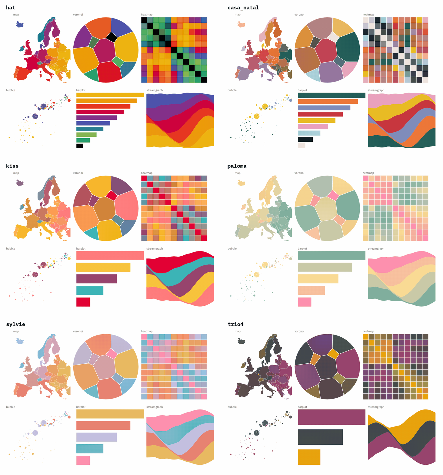
Try them yourself in the interactive palette explorer — switch between palettes, darken or brighten them, and check how they hold up under colour-vision deficiency.
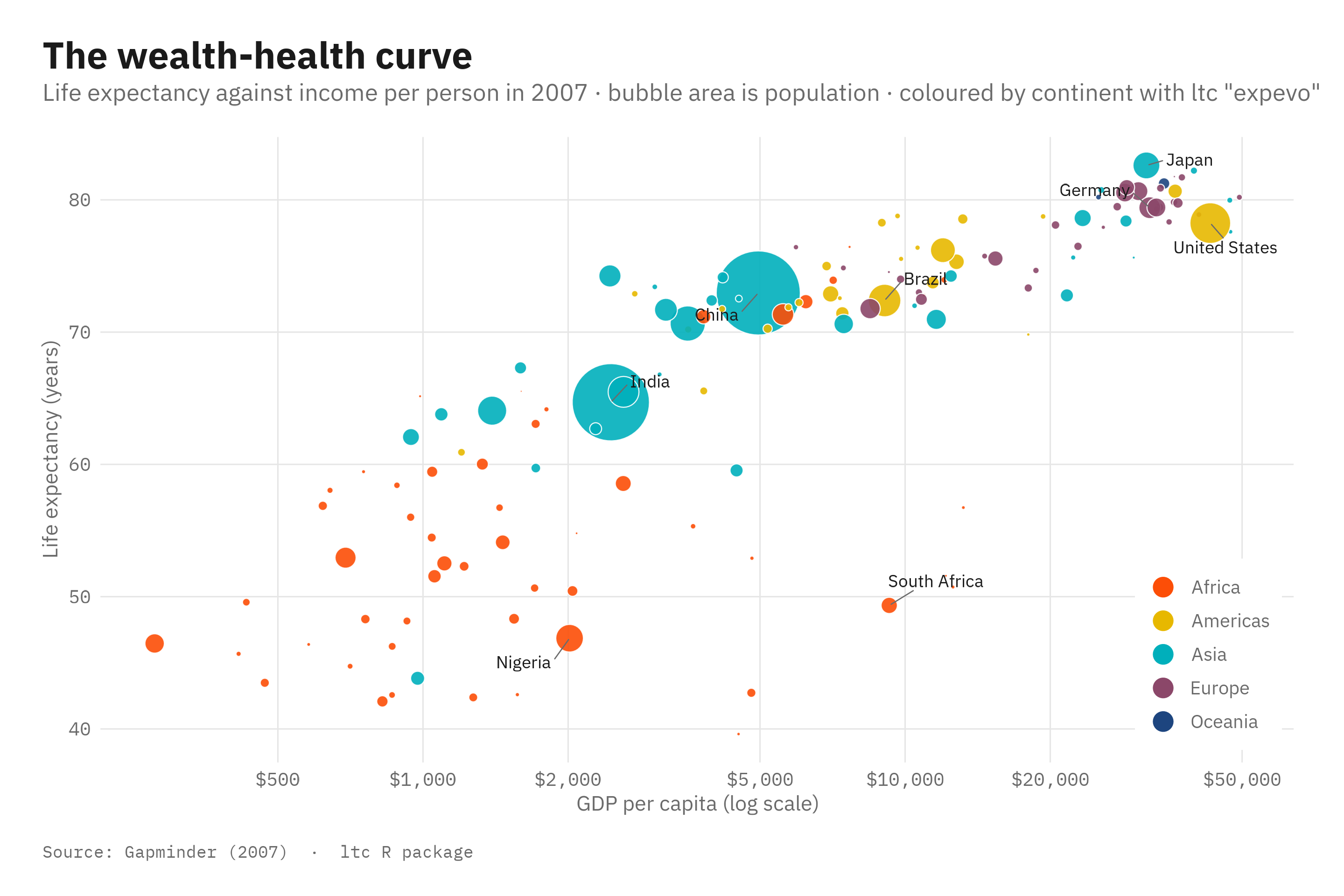
Two examples on real data. A discrete scale — life expectancy against income across the world in 2007, coloured by continent with the expevo palette:
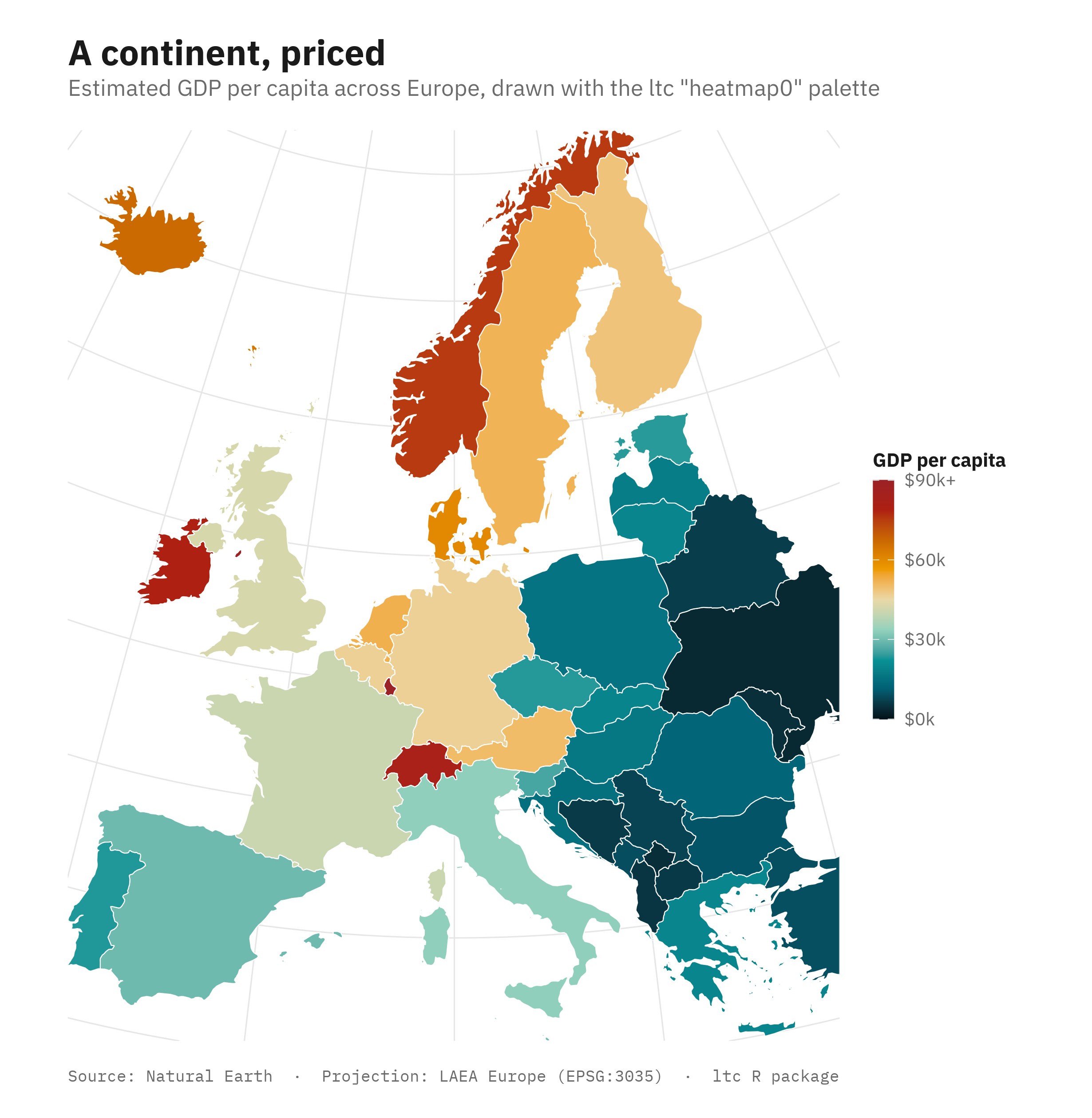
And a continuous scale — estimated GDP per capita across Europe, drawn with the heatmap0 palette:
Every function below follows the same pattern: what it is for, the arguments that matter (with their defaults), and a worked example.
The functions
ltc() — select a palette
What it’s for: picking a palette by name — with or without quotes, or from a variable holding the name — and printing it in the console with the actual colours visible.
| Argument | Default | What it does |
|---|---|---|
name |
— | The palette name: ltc(paloma), ltc("paloma"), or pal <- "paloma"; ltc(name = pal)
|
n |
all colours | How many colours to take |
type |
"discrete" |
"discrete" picks the first n; "continuous" interpolates a ramp of n
|
library(ltc)
names(palettes)
#>  [1] "paloma"     "maya"       "dora"       "ploen"      "olga"
#>  [6] "mterese"    "gaby"       "franscoise" "fernande"   "sylvie"
#> [11] "expevo"     "minou"      "kiss"       "hat"        "reading"
#> [16] "alger"      "trio1"      "trio2"      "trio3"      "trio4"
#> [21] "heatmap0"   "pantone23"  "remains"    "midnight"   "lincoln"
#> [26] "luminaries" "seafarer"   "shuggie"    "heatmap1"   "heatmap2"
#> [31] "heatmap3"   "casa_natal"

alger <- ltc("alger")
plot(alger)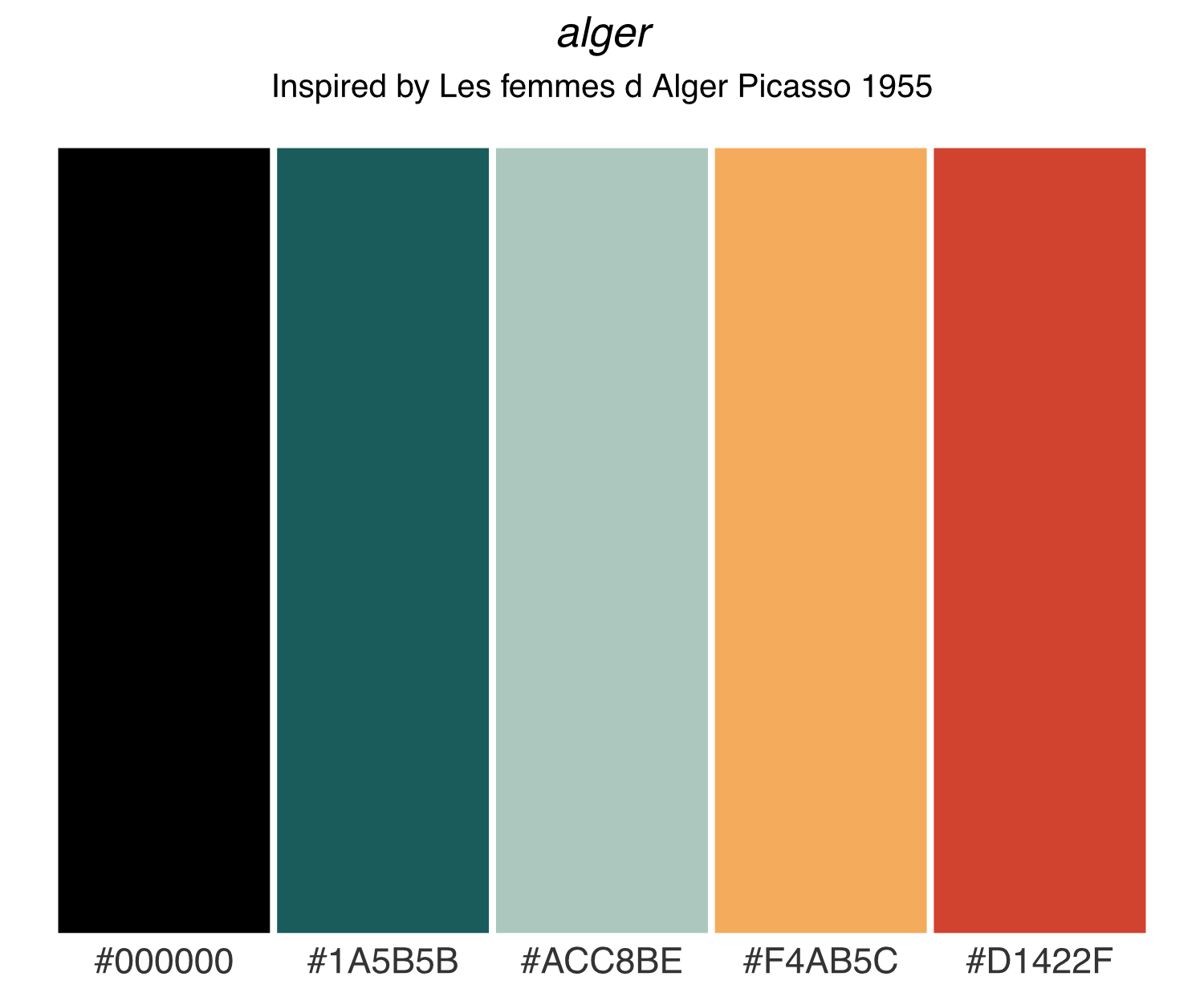
Each palette’s backstory lives in the bundled info data frame — plot() prints it as the subtitle.
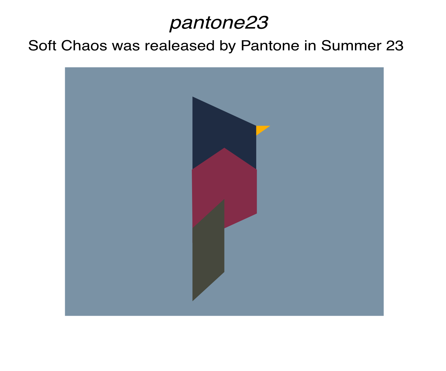
bird() — print a palette as a bird
What it’s for: the ltc signature — visualising a palette (of at least 5 colours) as a bird drawing:
scale_fill_ltc() / scale_colour_ltc() — ggplot2 scales
What they’re for: using a palette directly in ggplot2, exactly like scale_fill_viridis() — no scale_fill_manual(values = ...) needed. scale_color_ltc() is the same function under the US spelling.
| Argument | Default | What it does |
|---|---|---|
name |
— | Palette name, quoted or bare |
discrete |
TRUE |
FALSE builds a continuous gradient instead |
direction |
1 |
-1 reverses the palette |
library(ggplot2)

# discrete
ggplot(mtcars, aes(factor(cyl), mpg, fill = factor(cyl))) +
  geom_boxplot() +
  scale_fill_ltc(maya)

# continuous
ggplot(faithfuld, aes(waiting, eruptions, fill = density)) +
  geom_raster() +
  scale_fill_ltc(heatmap0, discrete = FALSE)

# reverse the palette
scale_colour_ltc(alger, direction = -1)
For other scale constructors, ltc_pal() returns a palette function of n:
ltc_pal(maya)(3)
#> [1] "#3d5a80" "#98c1d9" "#e0fbfc"
adjust_ltc() / desaturate_ltc() — tune a palette
What they’re for: darkening, lightening, or muting a palette without leaving the package.
| Argument | Default | What it does |
|---|---|---|
palette_name |
— | Palette name, quoted or bare |
amount |
0 / 0.5
|
adjust_ltc(): negative darkens, positive lightens; desaturate_ltc(): 0–1 mutes |
which |
all colours | Restrict to specific colour positions, e.g. c(1, 4)
|
adjust_ltc(maya, amount = -30)      # darker
adjust_ltc(maya, amount =  30)      # lighter
desaturate_ltc(maya, amount = 0.6)  # muted

# tune individual colours, or give each its own amount
adjust_ltc(maya, amount = -25, which = c(1, 4))
custom_adjust_ltc(maya, c(-40, -20, 0, 20, 40))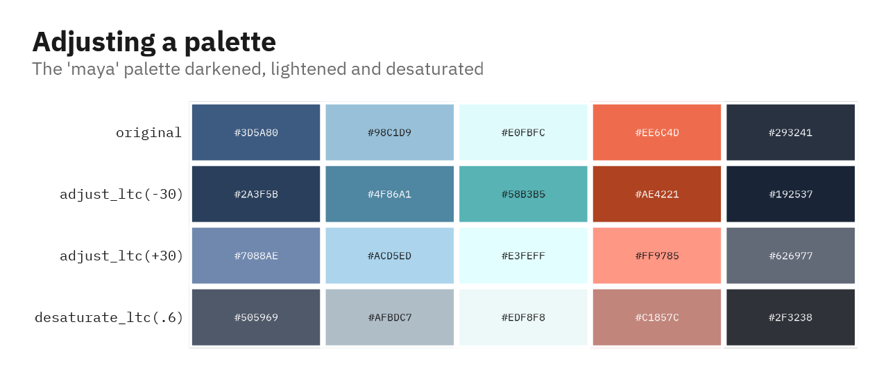
ltc_cvd() — check colour-vision accessibility
What it’s for: simulating how a palette looks to viewers with the three main types of colour-vision deficiency, so you can check that the colours stay distinct.
| Argument | Default | What it does |
|---|---|---|
name |
— | Palette name, quoted or bare |
severity |
1 |
Simulation strength, 0–1 |
labels |
TRUE |
Print the hex codes on the swatches |
ltc_cvd(maya)                     # normal + deuteranopia / protanopia / tritanopia
ltc_cvd("expevo", severity = 0.6) # milder simulation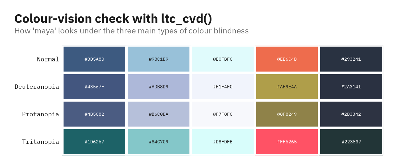
Palettes in action
A hexagon-density plot with a continuous heatmap0 ramp:
library(ggplot2)
pal <- ltc("heatmap0", 10, "continuous")

ggplot(data.frame(x = rnorm(1e4), y = rnorm(1e4)), aes(x = x, y = y)) +
  geom_hex() +
  coord_fixed() +
  scale_fill_gradientn(colours = pal) +
  theme_void()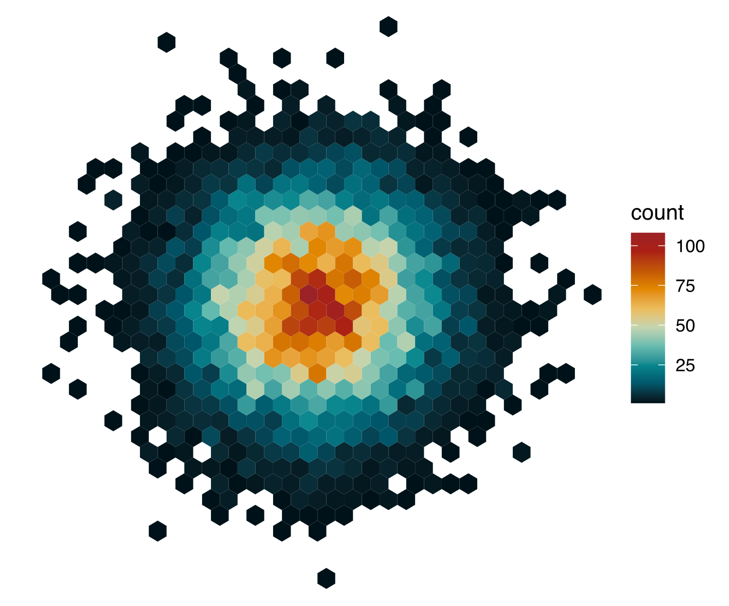
And a filled histogram from a 5-colour alger ramp:
pal <- ltc("alger", 5, "continuous")

ggplot(diamonds, aes(price, fill = cut)) +
  geom_histogram(binwidth = 500, position = "fill") +
  scale_fill_manual(values = pal) +
  theme_bw() +
  theme(panel.grid.major = element_blank(), panel.grid.minor = element_blank())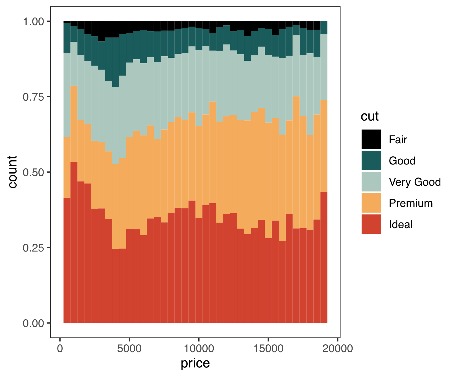
API reference
| Function | Purpose |
|---|---|
ltc() |
Select a palette by name (n, type = "discrete"/"continuous") |
plot() |
Print a palette as colour tiles, with its backstory |
bird() |
Print a palette as a bird drawing |
scale_fill_ltc() / scale_colour_ltc()
|
ggplot2 fill/colour scales (discrete, direction) |
ltc_pal() |
Palette function of n, for other scale constructors |
adjust_ltc() |
Darken (negative) or lighten (positive) colours |
custom_adjust_ltc() |
Per-colour adjustment amounts |
desaturate_ltc() |
Mute colours |
ltc_cvd() |
Simulate colour-vision deficiency |
palettes / info
|
The palette list and the backstories |
Contributions
The ltc package is developed and maintained by Loukas Theodosiou (theodosiou@evolbio.mpg.de). For the palettes I drew inspiration from the drawings and life of Pablo Picasso as well as from the following books:

ltc pairs naturally with its sibling packages ggvmap (Voronoi treemaps) and ggsynteny (synteny plots) — both accept every ltc palette by name.