Create a Volcano Plot — ggvolc • ggvolc

This function creates a volcano plot using ggplot2 based on provided datasets. It is particularly useful for visualizing differential gene expression data.

Usage

ggvolc(
  data1,
  data2 = NULL,
  size_var = NULL,
  p_value = 0.05,
  fc = 1,
  sig_col = c("padj", "pvalue"),
  label_top = NULL,
  label_dir = c("both", "up", "down", "each"),
  title = NULL,
  interactive = FALSE,
  not_sig_color = "#808080",
  down_reg_color = "#00798c",
  up_reg_color = "#d1495b",
  add_seg = FALSE
)

Arguments

data1: Data frame for the primary dataset. Accepts output from DESeq2 (results()), edgeR (topTags()), or limma (topTable()). Gene identifiers can live in a genes column or in the row names.
data2: Data frame for the secondary dataset (genes of interest). Uses the same auto-detection as data1. Default is NULL.
size_var: Variable for determining the size of points. Options are "log2FoldChange" and "pvalue". Default is NULL (fixed size).
p_value: Threshold for statistical significance. Default is 0.05.
fc: Fold change threshold for determining upregulated or downregulated genes. Default is 1.
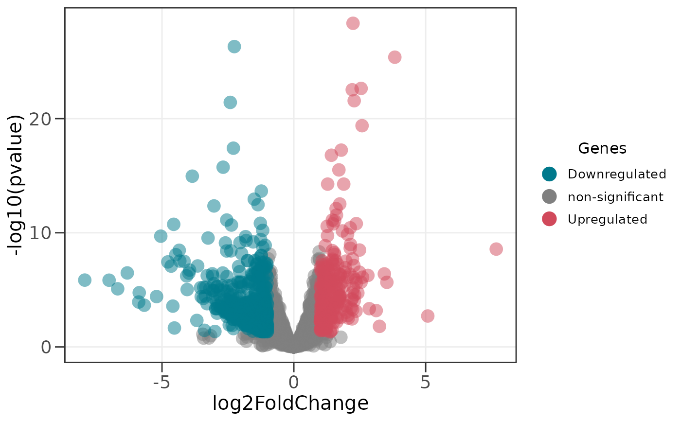
sig_col: Column used to call significance and to build the y-axis. Either "padj" (the adjusted p-value / FDR, the default and the recommended cutoff for calling hits in most DE workflows) or "pvalue" (the raw p-value). The y-axis and the significance segment follow this choice, so the plot stays internally consistent. When the default "padj" is used but the data has no adjusted-p column, ggvolc falls back to the raw p-value.
label_top: Optional integer. When supplied, the label_top most significant genes (smallest sig_col, among significant genes) are highlighted and labelled automatically, without building a separate data2. Combined with data2 if both are given. Default NULL.
label_dir: Direction to draw the label_top genes from. One of "both" (top N over all significant genes, the default), "up" (top N upregulated), "down" (top N downregulated), or "each" (top N upregulated and top N downregulated, i.e. up to 2N labels). Ignored when label_top is NULL.
title: Plot title. Default NULL (no title).
interactive: Logical. If TRUE, returns an interactive ggiraph girafe widget where hovering a point reveals the gene name and its statistics. Requires the optional ggiraph package. Default FALSE.
not_sig_color: Color for non-significant genes. Default is "#808080".
down_reg_color: Color for downregulated genes. Default is "#00798c".
up_reg_color: Color for upregulated genes. Default is "#d1495b".
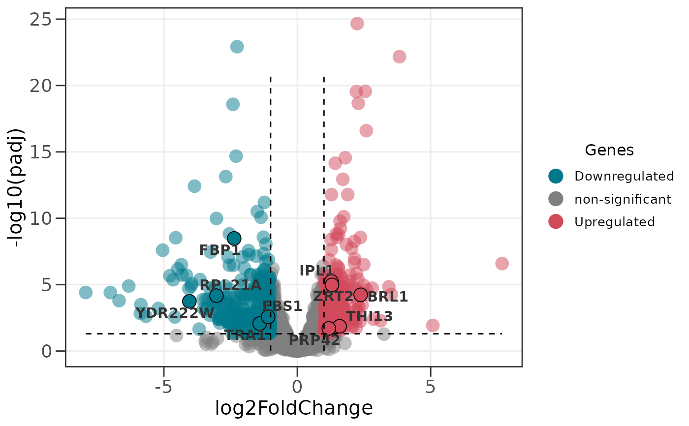
add_seg: Logical. If TRUE, dashed lines will be added to the plot indicating the p-value and fold change thresholds. Default is FALSE.

Value

A ggplot2 object displaying the volcano plot, or, when interactive = TRUE, a ggiraph girafe widget.

Details

Column names from DESeq2, edgeR, and limma are automatically detected and mapped internally, so you can pass the output of any of the three pipelines directly.

Examples

# Load example datasets included in the package
data(all_genes)
data(attention_genes)

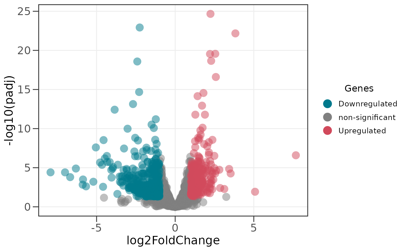
# Create a basic volcano plot with default settings
# Points are colored by significance (p < 0.05, |log2FC| > 1)
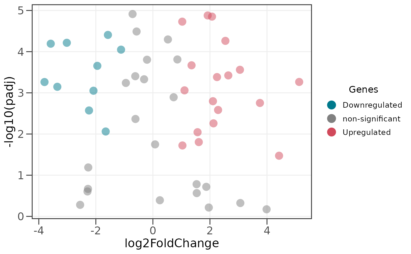
ggvolc(all_genes)


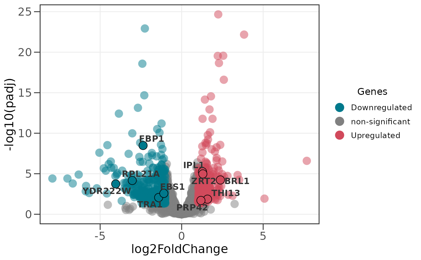
# Highlight specific genes of interest with labels
# These genes are shown with black borders and gene names
ggvolc(all_genes, attention_genes)


# Add dashed lines to indicate significance thresholds
ggvolc(all_genes, attention_genes, add_seg = TRUE)


# Significance is called on the adjusted p-value (FDR) by default;
# use the raw p-value instead with:
ggvolc(all_genes, sig_col = "pvalue")


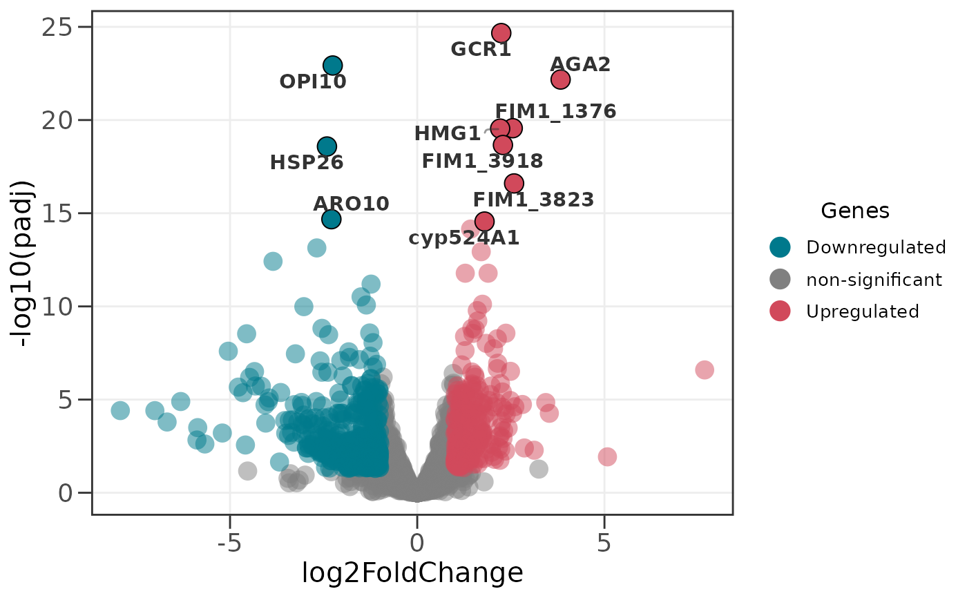
# Automatically label the 10 most significant genes
ggvolc(all_genes, label_top = 10)


# Label the top 10 upregulated genes only
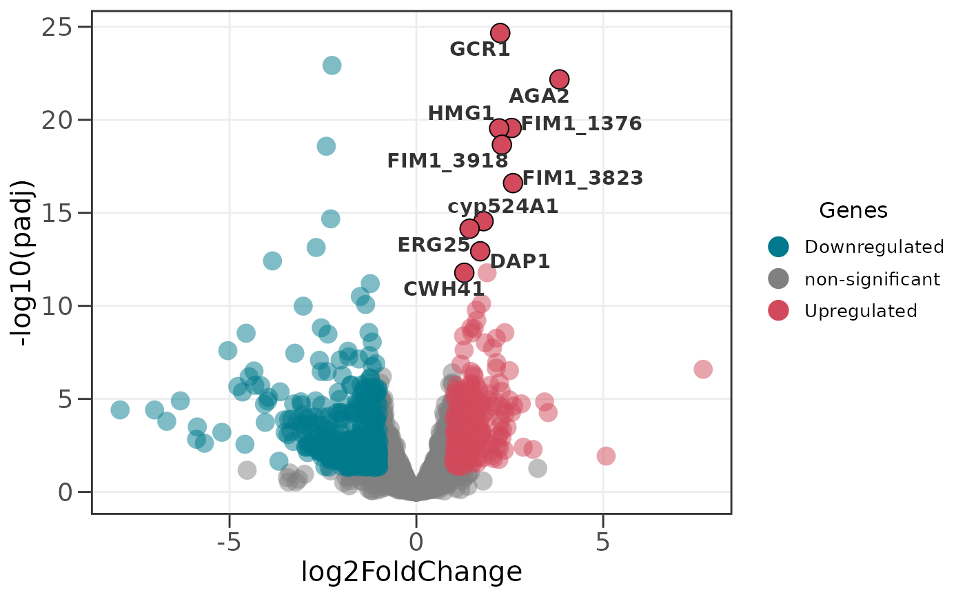
ggvolc(all_genes, label_top = 10, label_dir = "up")


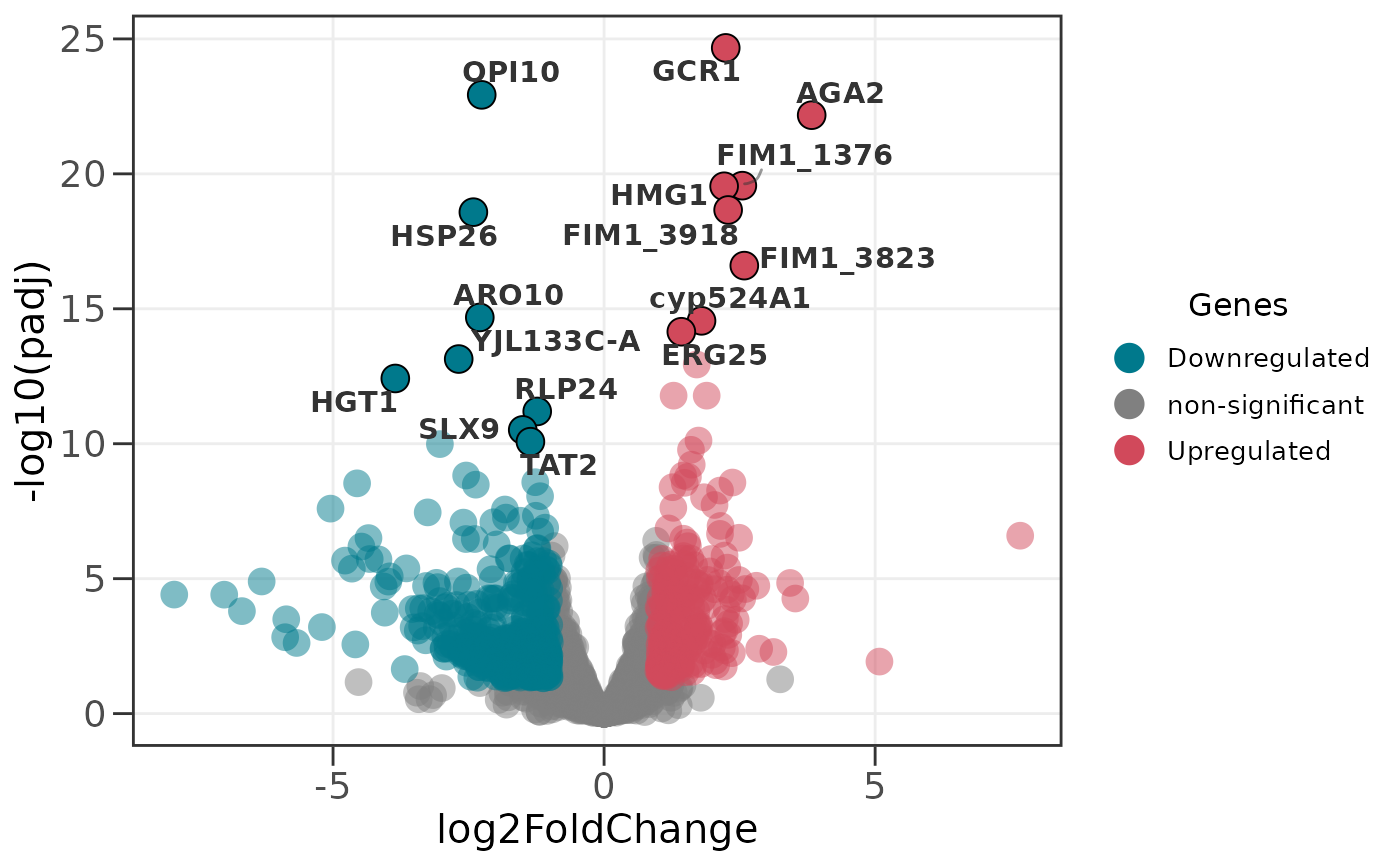
# Label the top 8 of each direction (up to 16 labels)
ggvolc(all_genes, label_top = 8, label_dir = "each")


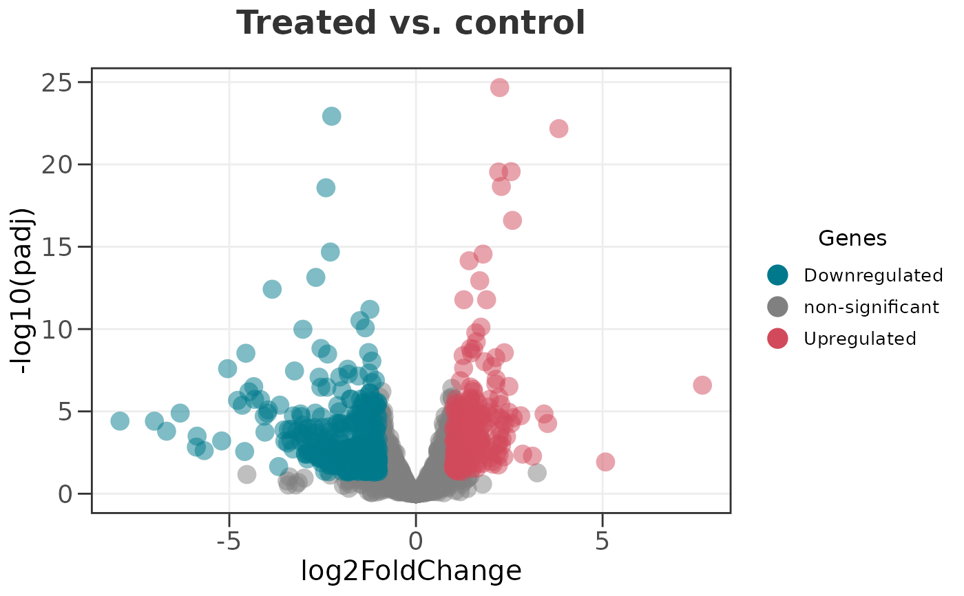
# Give the plot a title
ggvolc(all_genes, title = "Treated vs. control")


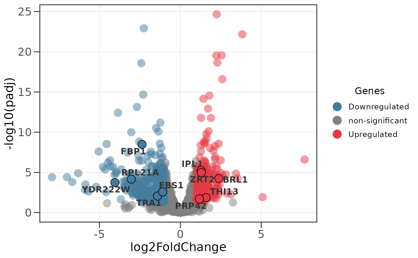
# Customize colors for up- and down-regulated genes
ggvolc(all_genes, attention_genes,
       up_reg_color = "#E63946",
       down_reg_color = "#457B9D")


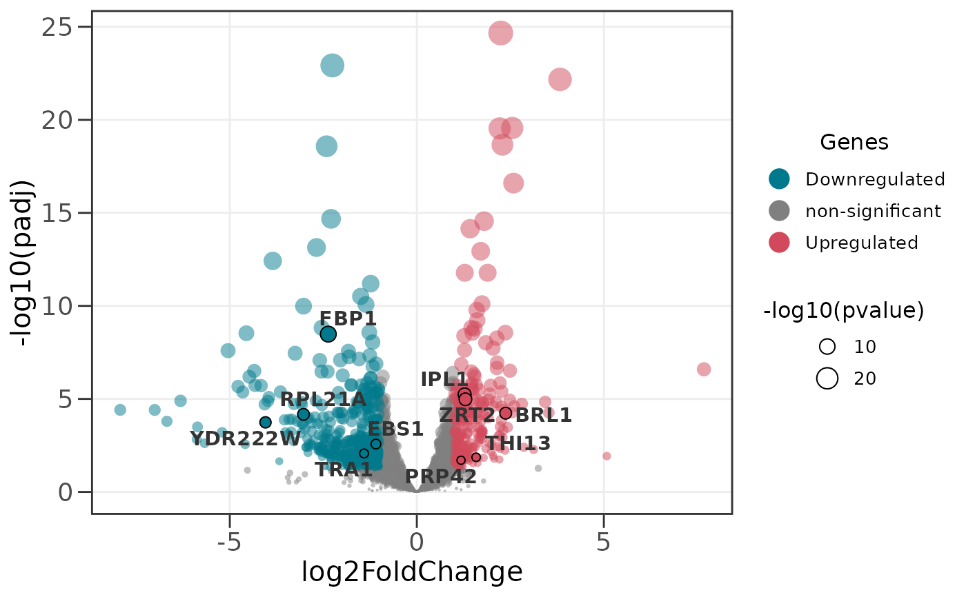
# Scale point size by p-value instead of default
ggvolc(all_genes, attention_genes, size_var = "pvalue")


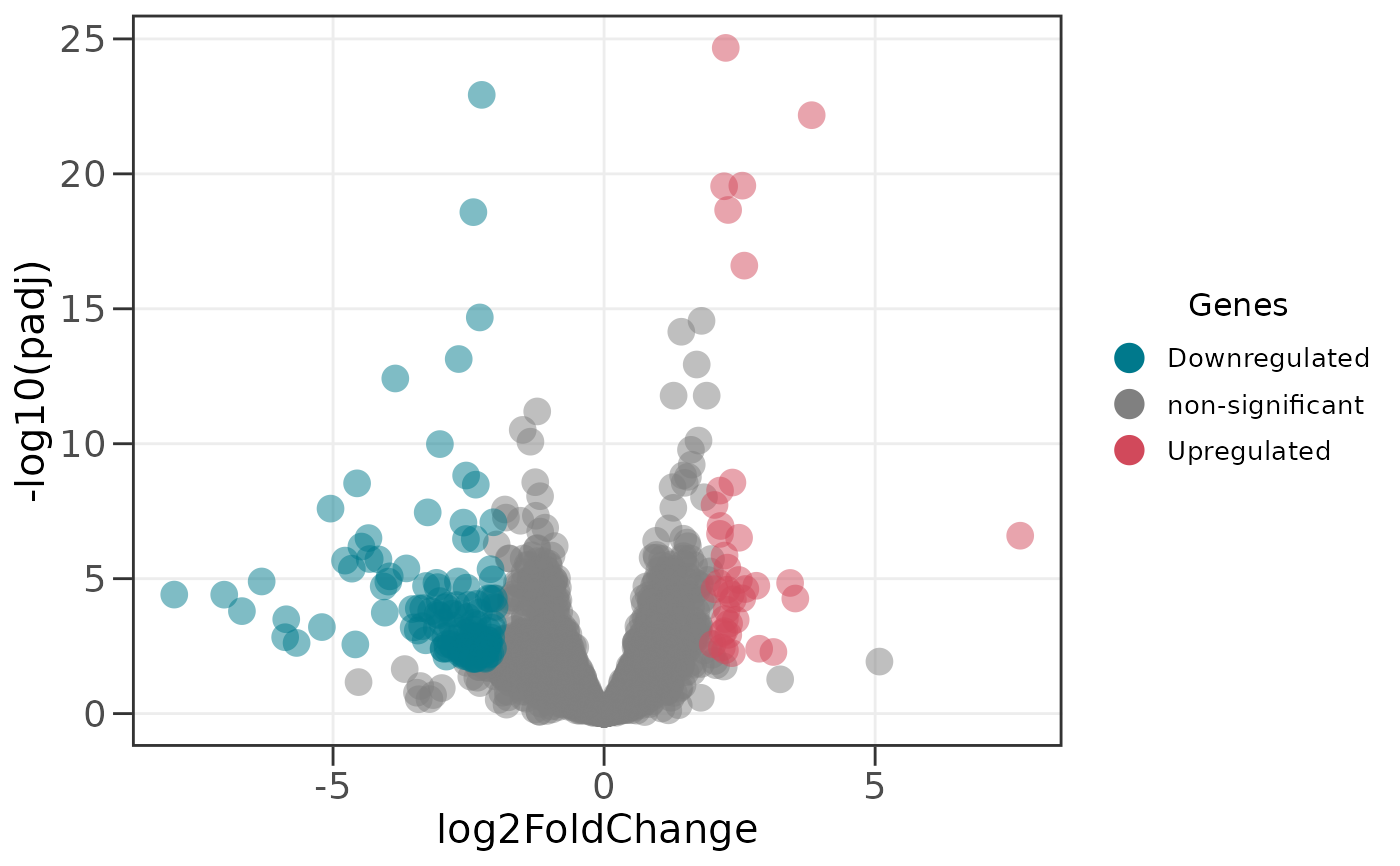
# Adjust significance thresholds (p-value and fold change)
ggvolc(all_genes, p_value = 0.01, fc = 2)


# edgeR-style input works directly
edger_df <- data.frame(
  genes = paste0("gene", 1:50),
  logFC = rnorm(50, 0, 2),
  logCPM = runif(50, 5, 15),
  PValue = 10^-runif(50, 0, 6),
  FDR = 10^-runif(50, 0, 5)
)
ggvolc(edger_df)


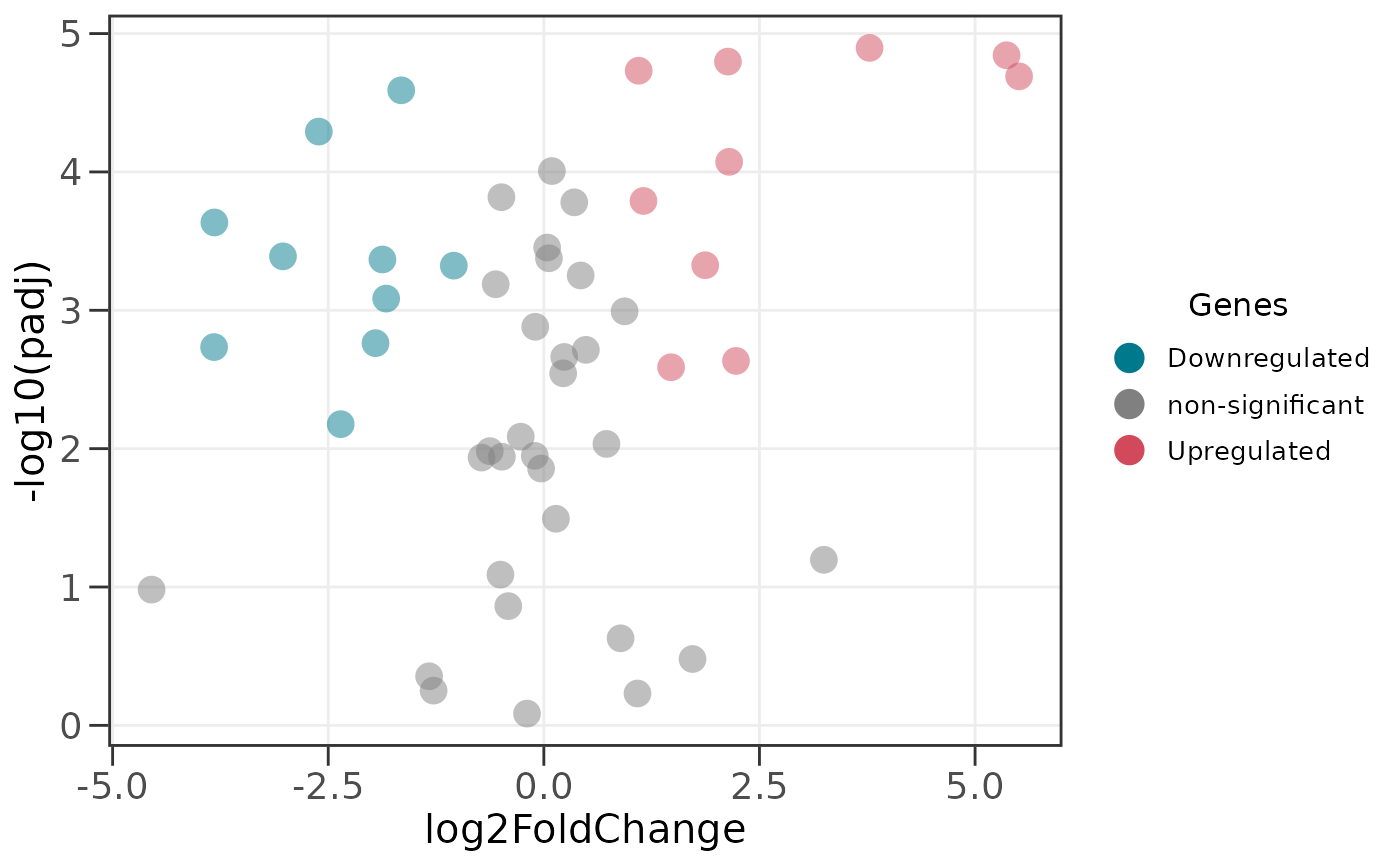# limma-style input works too
limma_df <- data.frame(
  genes = paste0("gene", 1:50),
  logFC = rnorm(50, 0, 2),
  AveExpr = runif(50, 5, 15),
  t = rnorm(50),
  P.Value = 10^-runif(50, 0, 6),
  adj.P.Val = 10^-runif(50, 0, 5)
)
ggvolc(limma_df)


if (FALSE) { # \dontrun{
# Interactive volcano (requires the ggiraph package): hover a point to
# see the gene name and its statistics
ggvolc(all_genes, attention_genes, interactive = TRUE)
} # }