Create Volcano Plots for Differential Gene Expression Data • ggvolc

Install the `ggvolc` package

Install the package using the following commands

# you can install ggvolc from CRAN 
install.packages("ggvolc")

# if you want to install the developmenetal version please use
devtools::install_github("loukesio/ggvolc")
# and load it
library(ggvolc)

How do I start?

ggvolc turns the results of a differential-expression analysis — from DESeq2, edgeR, or limma — into a clean, publication-ready volcano plot. From there you can highlight genes, auto-label the top hits, attach a gt table, or make the whole thing interactive. Start by loading the library and exploring the two example datasets that ship with the package:

library(ggvolc)
#> Welcome to ggvolc version 0.3.0 !
#>
#>                                 888
#>                                 888
#>                                 888
#>  .d88b.   .d88b.  888  888  .d88b.  888  .d8888b
#> d88P"88b d88P"88b 888  888 d88""88b 888 d88P"
#> 888  888 888  888 Y88  88P 888  888 888 888
#> Y88b 888 Y88b 888  Y8bd8P  Y88..88P 888 Y88b.
#>  "Y88888  "Y88888   Y88P    "Y88P"  888  "Y8888P
#>      888      888
#> Y8b d88P Y8b d88P
#>  "Y88P"   "Y88P"
#>

data(all_genes)     # data.frame that contains the output of differentially expressed genes
head(all_genes,5)   # have a look at the first 5 rows

#>       genes   baseMean log2FoldChange     lfcSE       stat       pvalue
#> 1      GCR1  7201.5782       2.244064 0.2004959  11.192564 4.434241e-29
#> 2     OPI10  1009.4171      -2.257454 0.2096469 -10.767889 4.880607e-27
#> 3      AGA2   249.1173       3.829474 0.3623263  10.569132 4.143136e-26
#> 4 FIM1_1376  5237.5035       2.550409 0.2560379   9.961059 2.256459e-23
#> 5      HMG1 10838.1037       2.214300 0.2229065   9.933763 2.968371e-23
#>           padj
#> 1 2.153711e-25
#> 2 1.185255e-23
#> 3 6.707736e-23
#> 4 2.739905e-20
#> 5 2.883475e-20


data(attention_genes)     # here is a data.frame with genes that I want to mention to the volcano plot
head(attention_genes,5)   # have a look at the first five rows
#>     genes   baseMean log2FoldChange     lfcSE      stat       pvalue
#> 1   THI13   480.5194       1.585811 0.5219706  3.038122 2.380572e-03
#> 2    FBP1 22710.8428      -2.366733 0.3533032 -6.698871 2.100354e-11
#> 3    TRA1  4491.1343      -1.410696 0.4384316 -3.217595 1.292700e-03
#> 4 YDR222W   591.2289      -4.045918 0.9133881 -4.429572 9.442026e-06
#> 5    BRL1  4434.7712       2.375919 0.5037264  4.716686 2.397176e-06
#>           padj
#> 1 1.371582e-02
#> 2 3.290780e-09
#> 3 8.565681e-03
#> 4 1.819838e-04
#> 5 5.850796e-05

^{Created on 2023-08-11 with reprex v2.0.2}

1. Plot a simple volcano plot!

Pass a single data frame and every gene is coloured by significance — down, up, or not significant.

ggvolc(all_genes)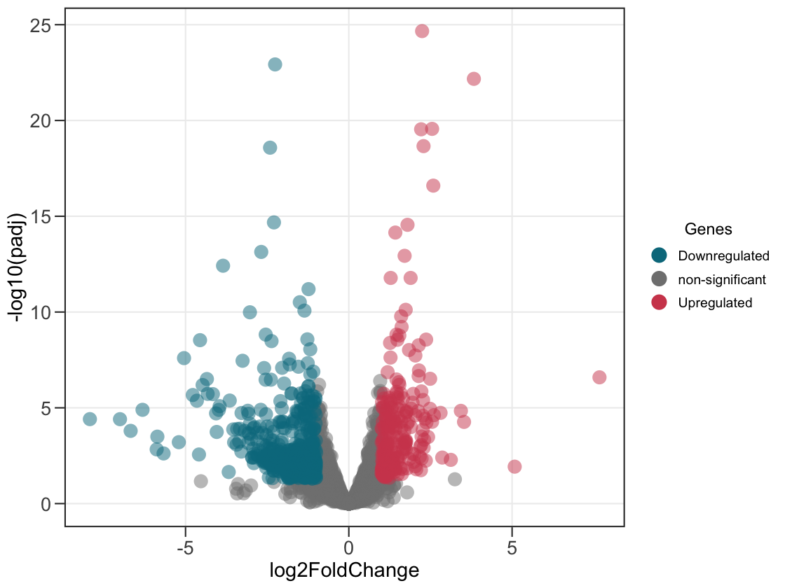

2. Add the genes of attention.

Supply a second data frame to outline and label the genes you care about.

ggvolc(all_genes, attention_genes)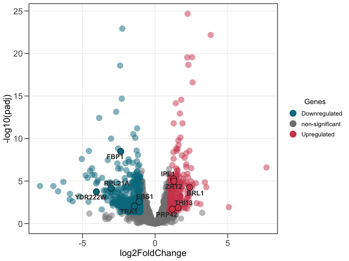

3. Add segments to indicate areas of significance.

Turn on add_seg to draw the fold-change and significance thresholds.

ggvolc(all_genes, attention_genes, add_seg = TRUE) +
  labs(title="Add segments of significance")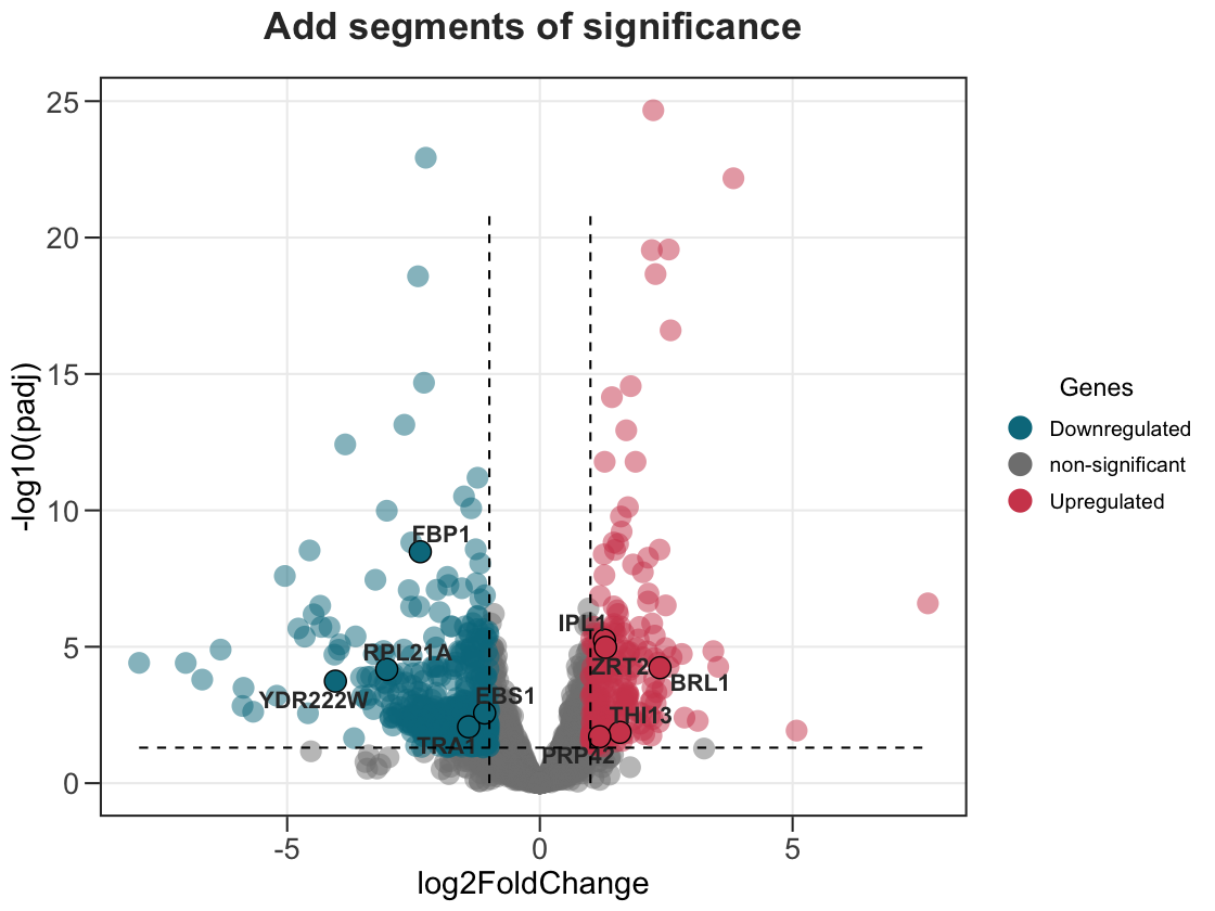

4. Indicate the size of point based on the log2FoldChange column.

Scale point size by effect size with size_var = "log2FoldChange".

ggvolc(all_genes, attention_genes, size_var = "log2FoldChange", add_seg = TRUE)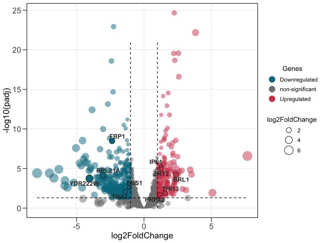

5. Indicate the size of the point based on the pvalue.

Or scale it by significance with size_var = "pvalue".

ggvolc(all_genes, attention_genes, size_var = "pvalue", add_seg = TRUE)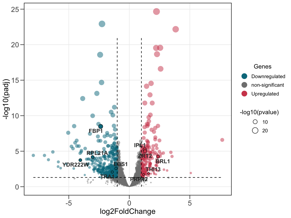

6. Add a table with the genes of interest.

plot <- ggvolc(all_genes, attention_genes, add_seg = TRUE) +
  labs(title="Add a table with the genes of interest")

plot %>%
  genes_table(attention_genes)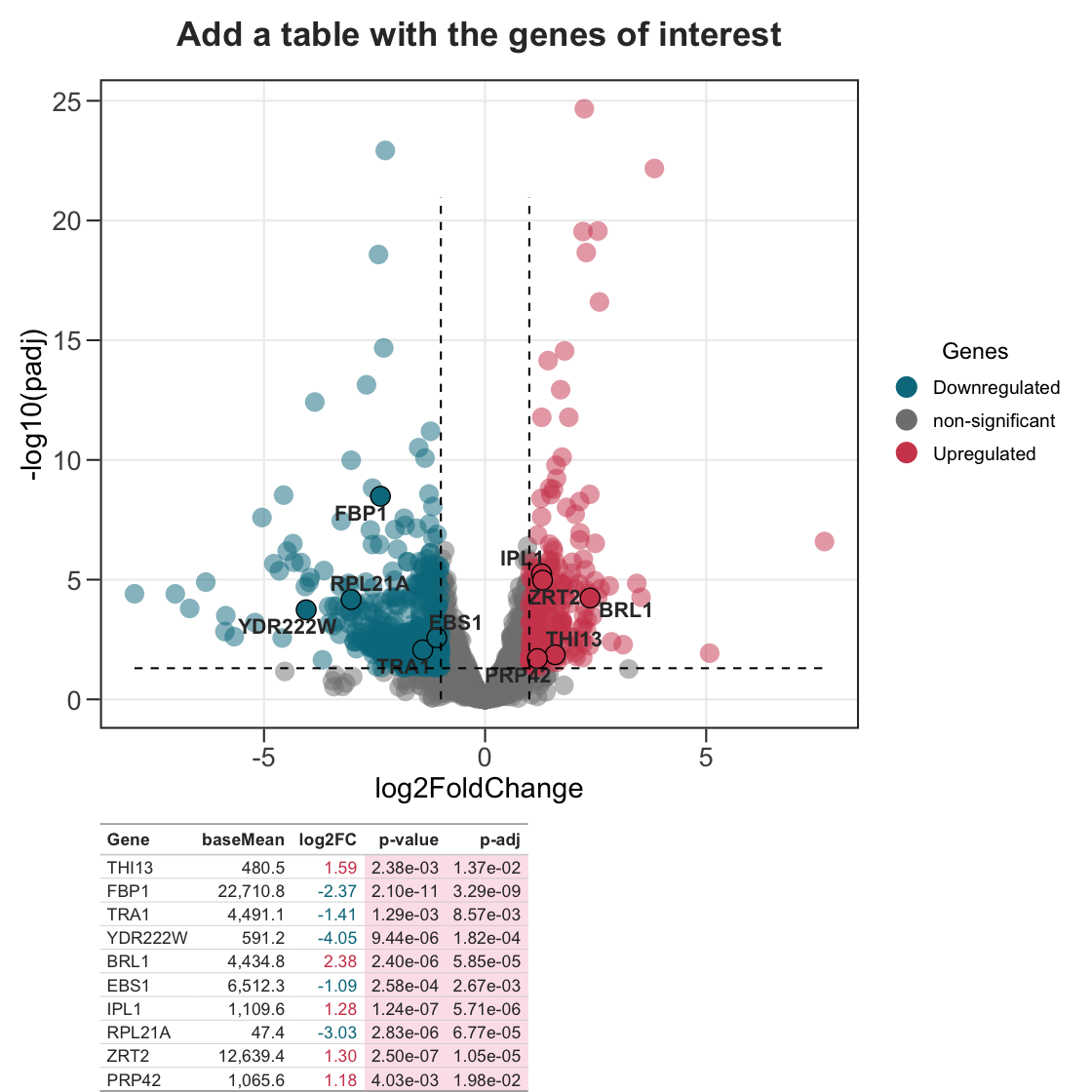

The gene table is rendered with gt and composed with patchwork, so the result is a single object you can style further or save with ggplot2::ggsave().

Instead of curating your own set of genes, you can let genes_table() pick the most significant ones automatically with top_n. Pass the full DE table and it selects the top genes by sig_col (defaults to padj, falling back to pvalue). Use dir = "each" to take the top N up- and down-regulated genes.

plot_top <- ggvolc(all_genes, label_top = 10, add_seg = TRUE) +
  labs(title = "Top 10 most significant genes")

plot_top %>%
  genes_table(all_genes, top_n = 10)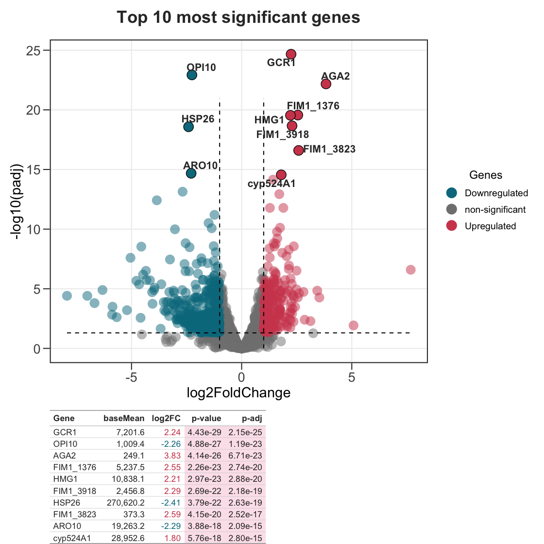

7. Works with DESeq2, edgeR, and limma out of the box

ggvolc() and genes_table() accept the output of all three major differential-expression pipelines directly — column names are auto-detected and mapped internally, so no manual renaming is needed. Gene identifiers held in row names (as edgeR/limma often do) are promoted to a genes column automatically.

Pipeline	Fold change	p-value	adjusted p	expression
DESeq2 (`results()`)	`log2FoldChange`	`pvalue`	`padj`	`baseMean`
edgeR (`topTags()`)	`logFC`	`PValue`	`FDR`	`logCPM`
limma (`topTable()`)	`logFC`	`P.Value`	`adj.P.Val`	`AveExpr`

The package ships edger_genes, an example topTags()-style table, so you can see this directly. In your own analysis you would pass the real thing:

# edgeR: pass topTags()$table straight in
edger_res <- as.data.frame(edgeR::topTags(qlf, n = Inf))
ggvolc(edger_res)

data(edger_genes)          # an edgeR topTags()-style table (genes in the rownames)
head(edger_genes, 3)
#>           logFC  logCPM       PValue          FDR
#> GCR1   2.244064 12.8143 4.434241e-29 2.153711e-25
#> OPI10 -2.257454  9.9807 4.880607e-27 1.185255e-23
#> AGA2   3.829474  7.9665 4.143136e-26 6.707736e-23

ggvolc(edger_genes, label_top = 8, add_seg = TRUE, title = "edgeR input")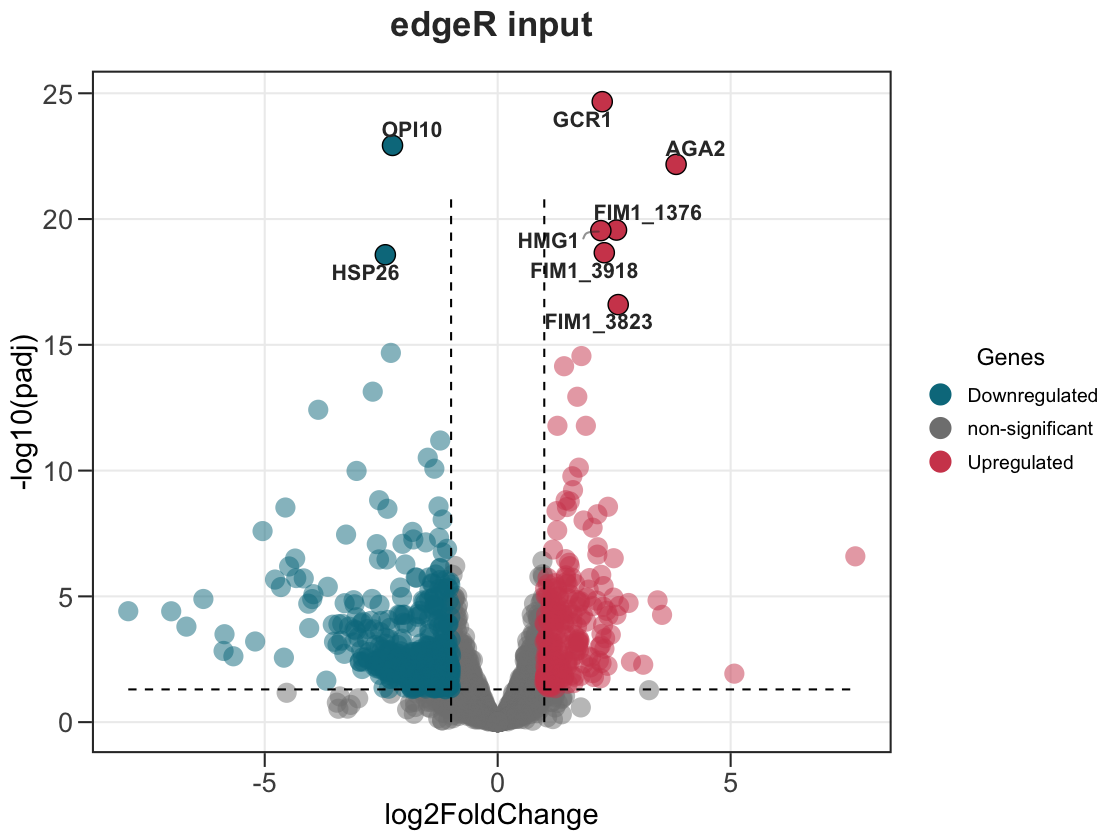

8. Significance on the adjusted p-value (FDR) — the default

ggvolc() calls significance on the adjusted p-value (FDR) by default — the right cutoff for most DE workflows — and the y-axis and the significance line follow along, so the plot stays consistent. Prefer the raw p-value? Set sig_col = "pvalue".

ggvolc(all_genes, add_seg = TRUE)   # significance on padj (FDR) by default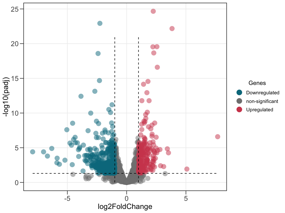

If your table has no adjusted-p column, ggvolc automatically falls back to the raw p-value.

ggvolc() is also robust to p-values of exactly 0 (which DESeq2/edgeR can emit for the strongest genes): instead of silently dropping them, their -log10 value is capped so they stay pinned near the top of the plot.

9. Automatically label the top genes

No need to build a separate data frame — label_top highlights and labels the N most significant genes for you, and label_dir lets you pick the direction.

# top 10 overall
ggvolc(all_genes, label_top = 10, add_seg = TRUE, title = "Top 10 hits")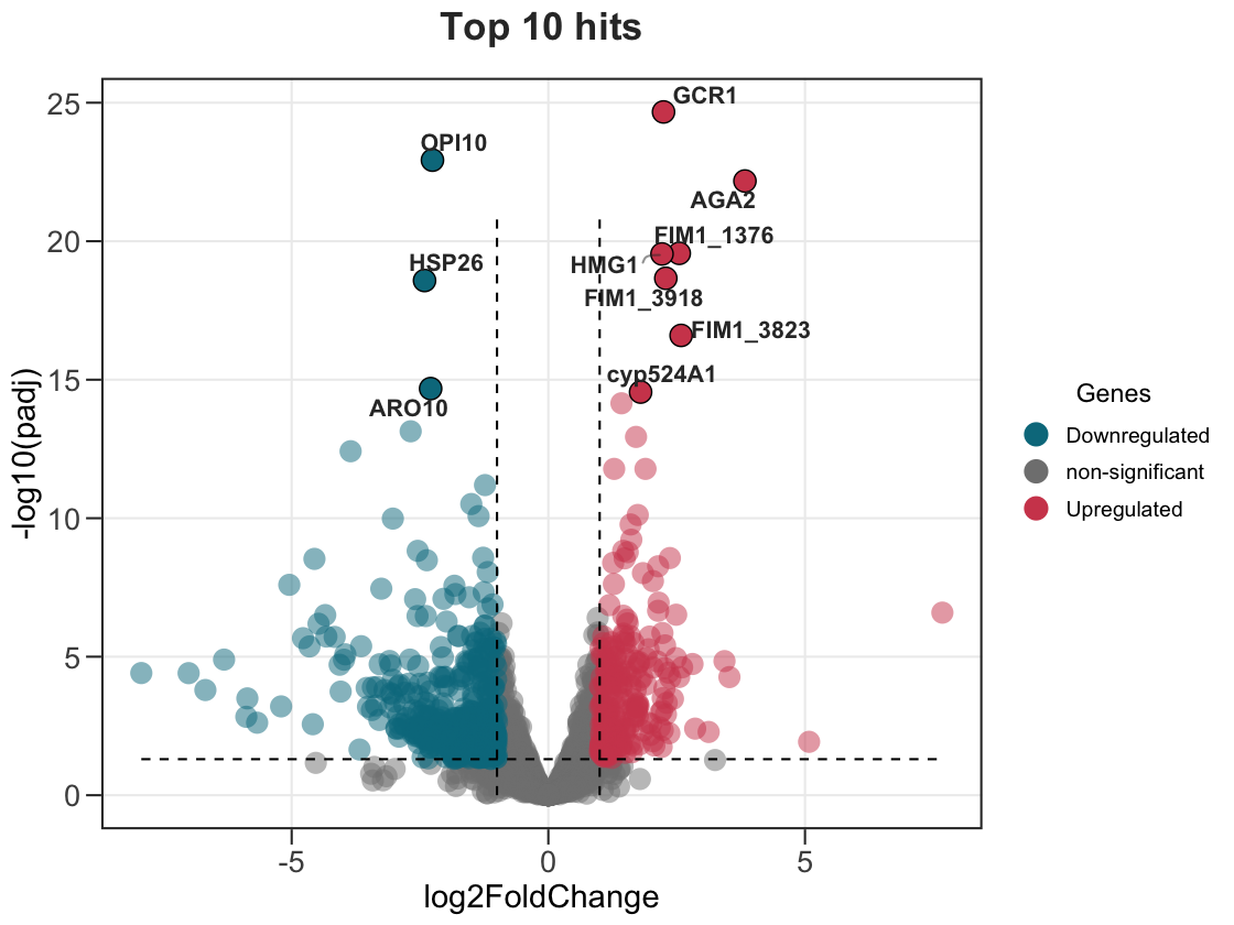

# top 8 up- and top 8 down-regulated
ggvolc(all_genes, label_top = 8, label_dir = "each", add_seg = TRUE,
       title = "Top 8 up + 8 down")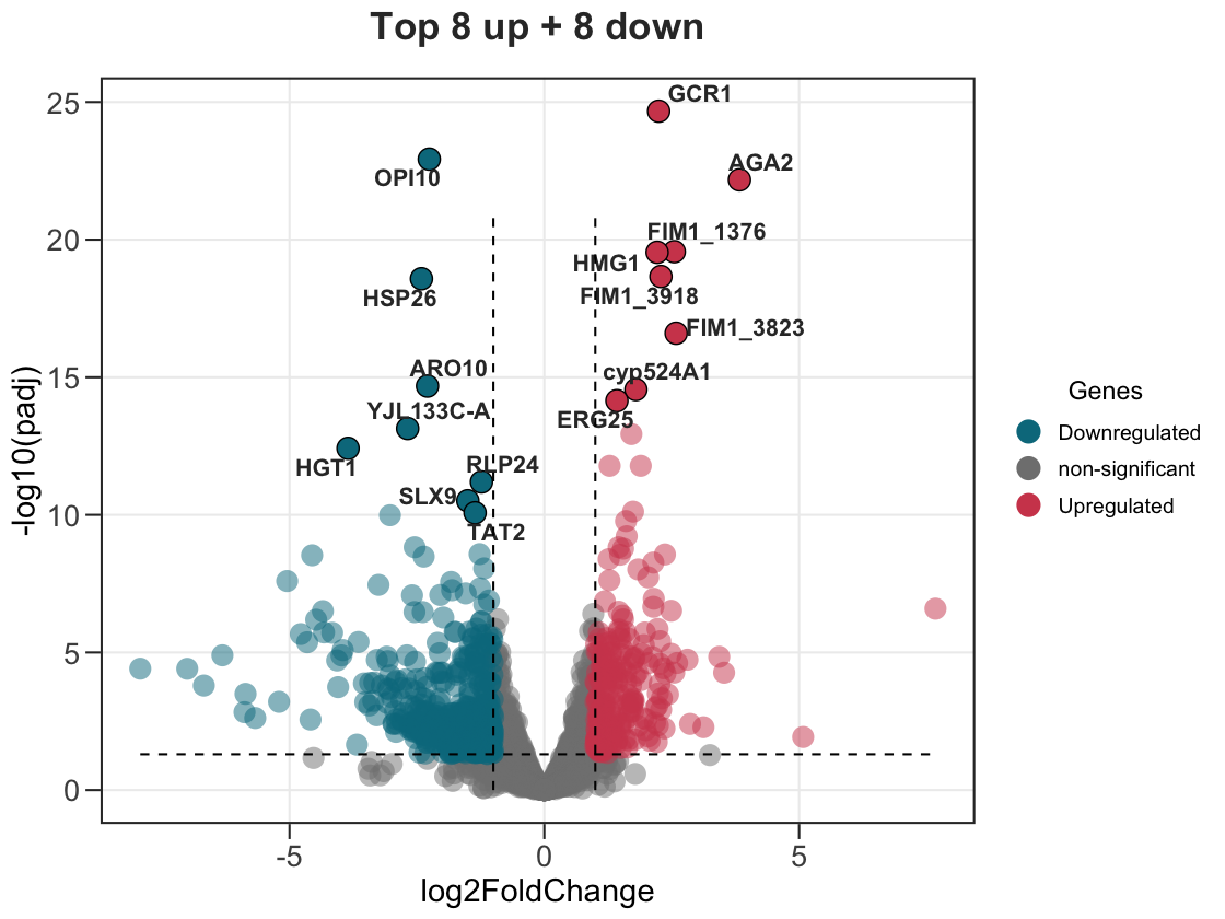

label_dir accepts "both" (default), "up", "down", or "each".

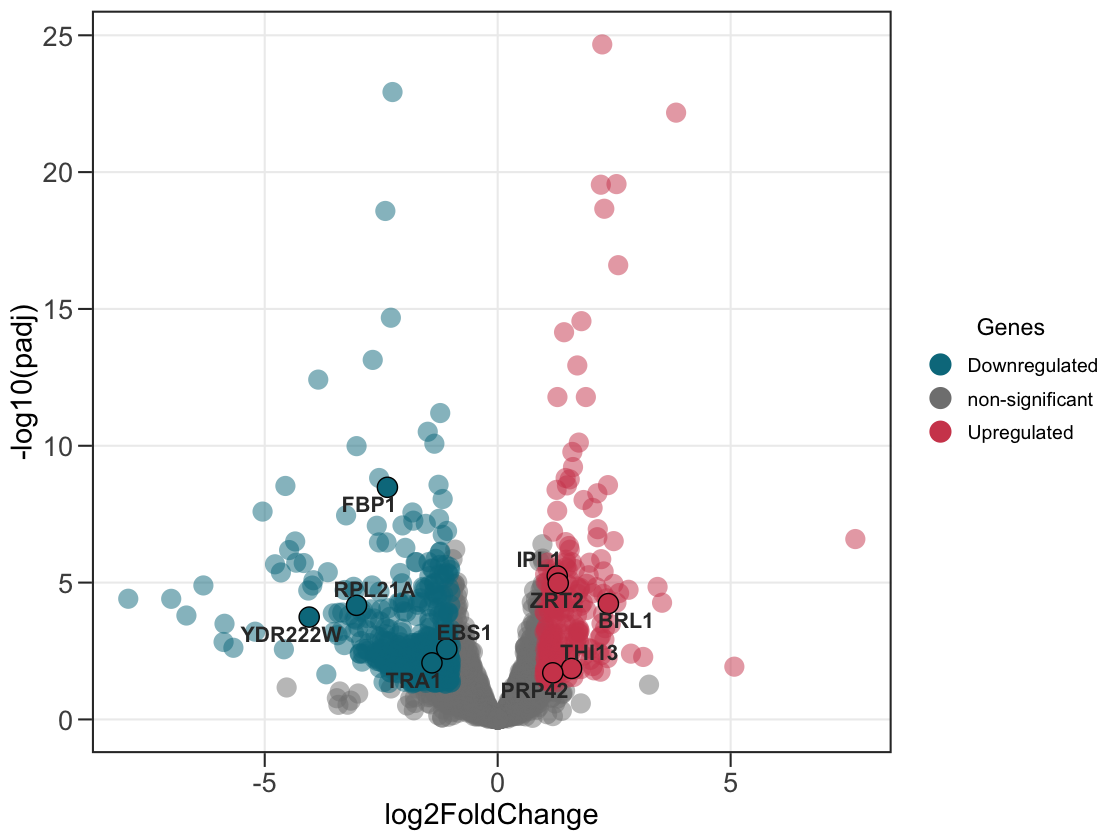
10. Make it interactive

Set interactive = TRUE to get an ggiraph widget — hover any point to see the gene name and its statistics. ggiraph is an optional dependency (install it with install.packages("ggiraph")).

ggvolc(all_genes, attention_genes, interactive = TRUE)

Note: GitHub can’t run the widget, so the image below is a static preview. The live, hover-to-inspect version runs in RStudio and on the package website.

Learn more

📖 Package website — full function reference and a getting-started article with every example (including the live interactive volcano).
🐳 Docker image — docker pull ghcr.io/loukesio/ggvolc:latest for a ready-to-run RStudio environment with ggvolc pre-installed.
🐛 Issues & questions — bug reports and feature requests are welcome.

Install the ggvolc package