Getting started with ggvolc • ggvolc

ggvolc turns the output of a differential-expression (DE) analysis into a polished, publication-ready volcano plot. It accepts the output of DESeq2, edgeR, and limma directly, highlights and labels genes of interest, combines the plot with a gt table, and can render an interactive version with ggiraph.

library(ggvolc)

The example data

The package ships with two data frames. all_genes is a complete DESeq2-style result table; attention_genes is a small subset of genes you might want to highlight.

data(all_genes)
data(attention_genes)

head(all_genes)
#>       genes   baseMean log2FoldChange     lfcSE       stat       pvalue
#> 1      GCR1  7201.5782       2.244064 0.2004959  11.192564 4.434241e-29
#> 2     OPI10  1009.4171      -2.257454 0.2096469 -10.767889 4.880607e-27
#> 3      AGA2   249.1173       3.829474 0.3623263  10.569132 4.143136e-26
#> 4 FIM1_1376  5237.5035       2.550409 0.2560379   9.961059 2.256459e-23
#> 5      HMG1 10838.1037       2.214300 0.2229065   9.933763 2.968371e-23
#> 6 FIM1_3918  2456.8070       2.288243 0.2356228   9.711467 2.694309e-22
#>           padj
#> 1 2.153711e-25
#> 2 1.185255e-23
#> 3 6.707736e-23
#> 4 2.739905e-20
#> 5 2.883475e-20
#> 6 2.181043e-19

A basic volcano plot

Passing a single data frame colours every gene by significance. By default a gene is called significant when its adjusted p-value (FDR) is below 0.05 and its |log2FoldChange| exceeds 1.

ggvolc(all_genes)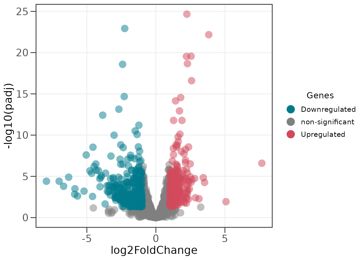

Highlighting genes of interest

Supply a second data frame and those genes are drawn with a black outline and labelled.

ggvolc(all_genes, attention_genes, add_seg = TRUE)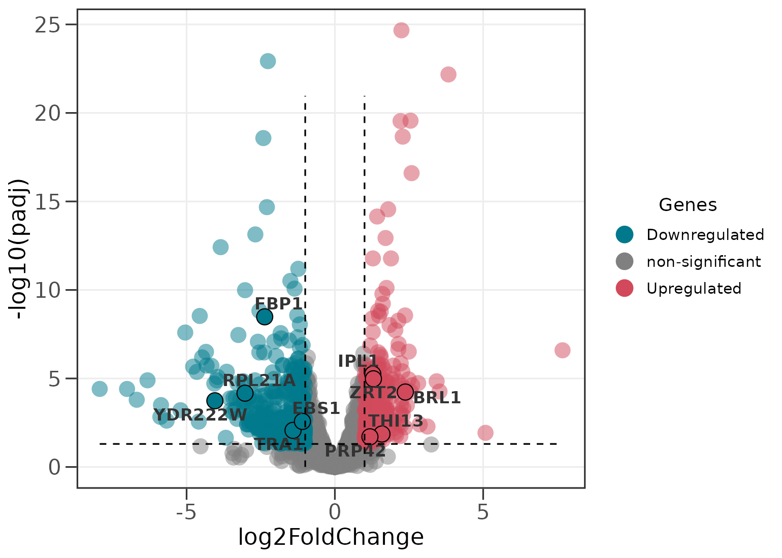

The add_seg = TRUE argument adds dashed guides at the fold-change and significance thresholds.

Labelling the top genes automatically

You usually do not want to build a separate data frame just to label a handful of hits. label_top picks the most significant genes for you, and label_dir controls the direction they are drawn from.

# the 10 most significant genes overall
ggvolc(all_genes, label_top = 10, add_seg = TRUE, title = "Top 10 hits")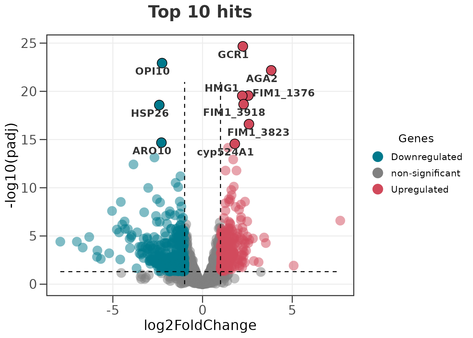

# the top 8 up- and top 8 down-regulated genes
ggvolc(all_genes, label_top = 8, label_dir = "each",
       add_seg = TRUE, title = "Top 8 up + 8 down")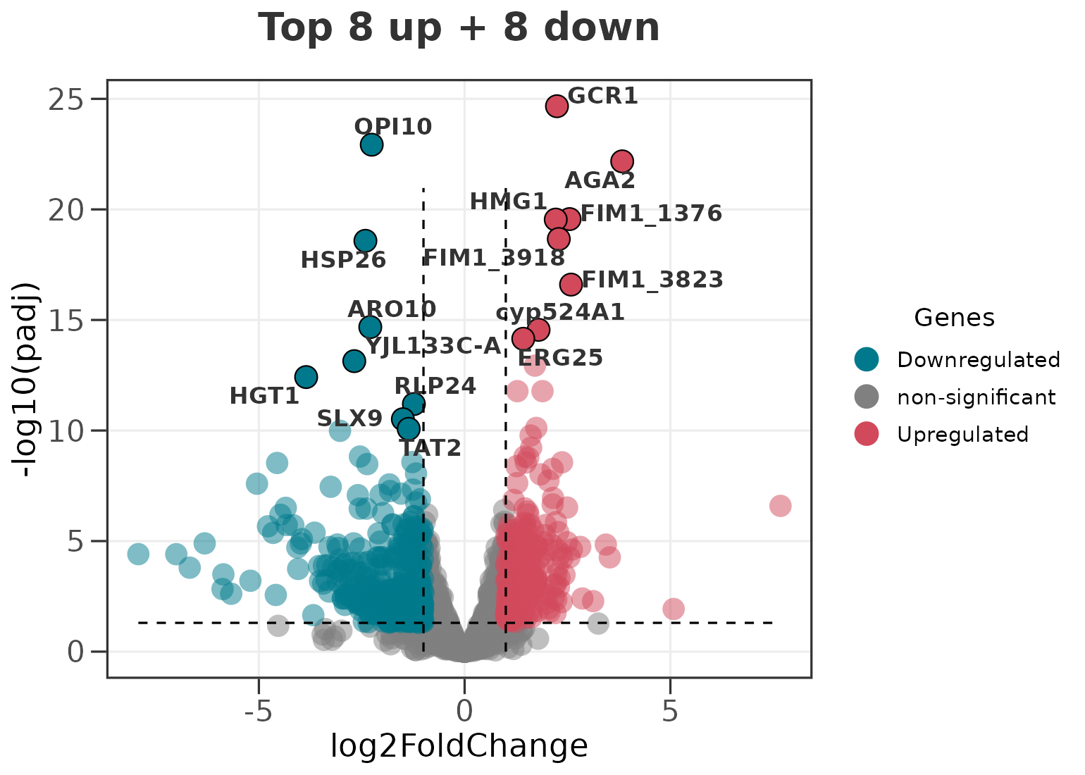

label_dir accepts "both" (the default), "up", "down", and "each".

Calling significance on the FDR (or the raw p-value)

ggvolc() calls significance on the adjusted p-value (padj) by default, which is the right cutoff for most DE workflows. The y-axis and the significance line follow the choice, so the plot stays internally consistent. Switch to the raw p-value with sig_col = "pvalue".

ggvolc(all_genes, sig_col = "pvalue", add_seg = TRUE,
       title = "Significance on the raw p-value")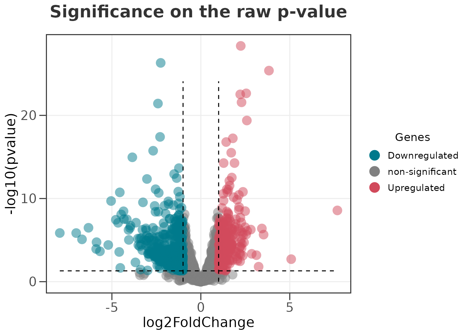

ggvolc() is also robust to p-values of exactly 0 (which DESeq2 and edgeR can emit for the strongest genes): rather than dropping those points, their -log10 value is capped so they stay near the top of the plot.

Scaling point size

Point size can encode either the fold change or the significance.

ggvolc(all_genes, attention_genes, size_var = "log2FoldChange", add_seg = TRUE)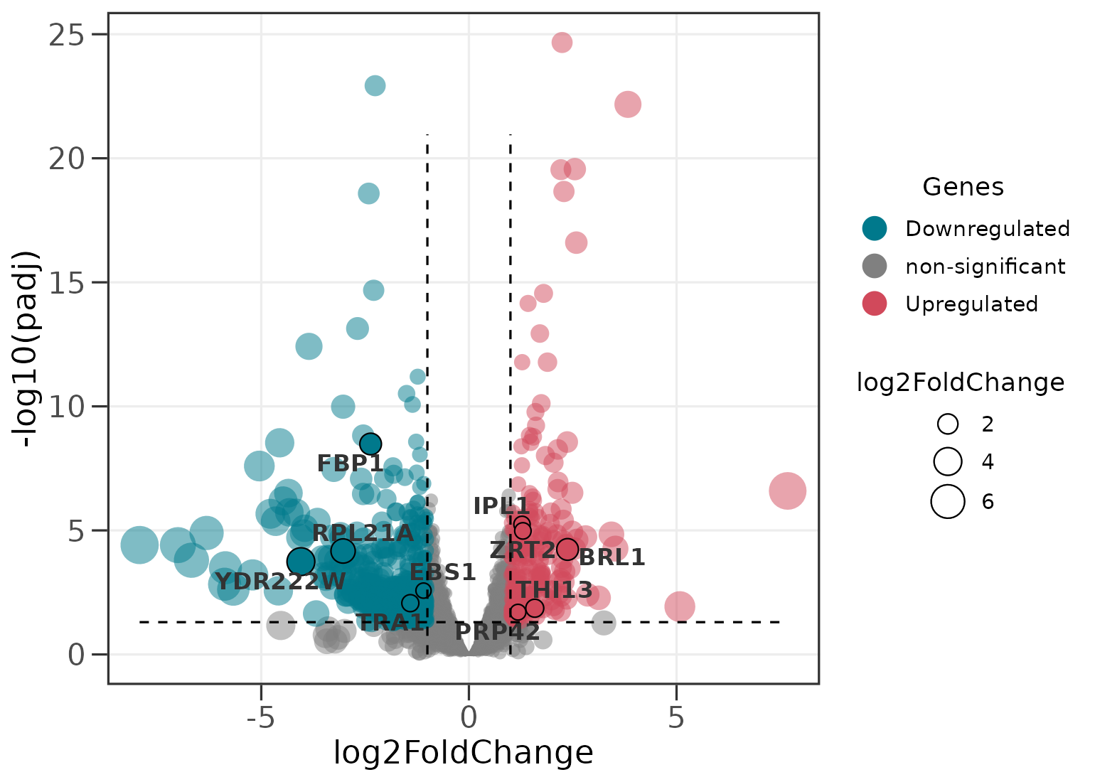

Adding a gene table

genes_table() composes the volcano plot with a gt table of the highlighted genes using patchwork. The result is a single object you can save with ggplot2::ggsave().

p <- ggvolc(all_genes, attention_genes, add_seg = TRUE)
genes_table(p, attention_genes)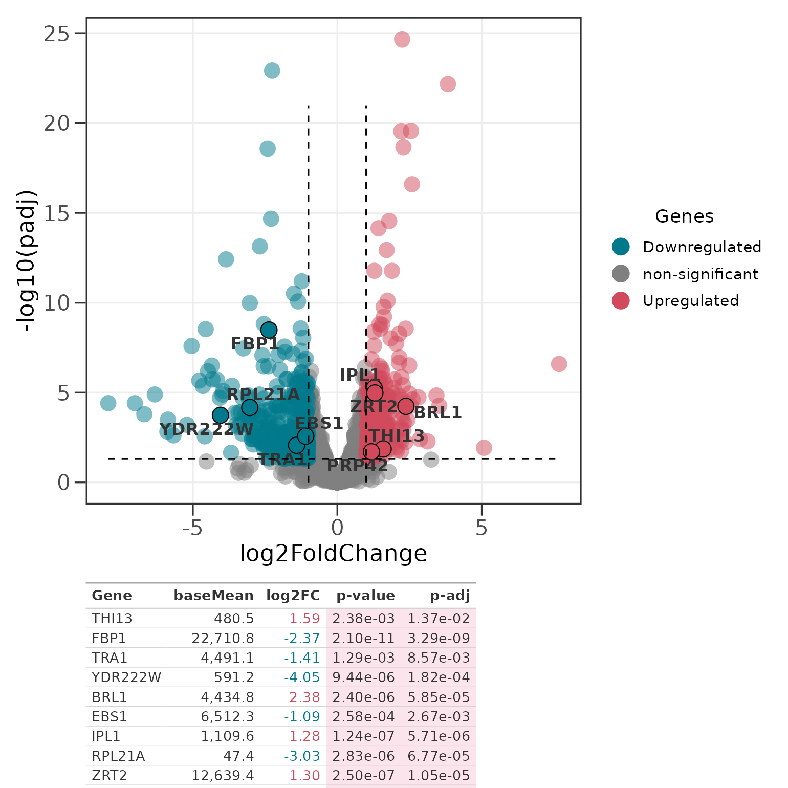

To tabulate the most significant genes without curating them yourself, pass the full DE table and a top_n. Genes are ranked by sig_col (padj by default, falling back to pvalue); dir = "each" takes the top N up- and down-regulated genes.

p_top <- ggvolc(all_genes, label_top = 10, add_seg = TRUE)
genes_table(p_top, all_genes, top_n = 10)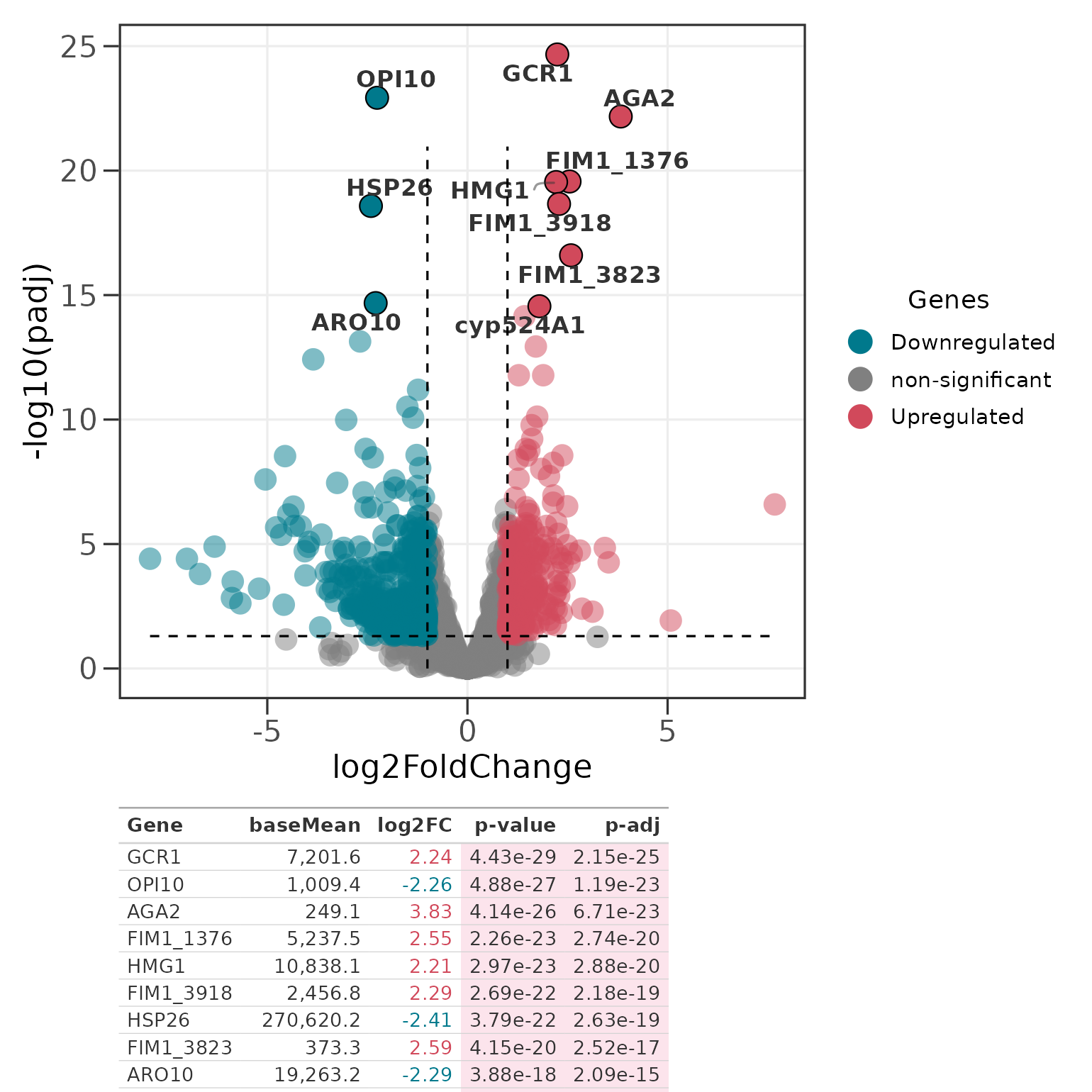

Works with DESeq2, edgeR, and limma

Column names from all three pipelines are detected and mapped automatically, so you can pass their output straight in. Gene identifiers held in the row names (as edgeR and limma often do) are promoted to a genes column for you.

The package ships edger_genes, an example topTags()-style table with the gene identifiers in the row names, so you can try this right away:

data(edger_genes)
head(edger_genes, 3)
#>           logFC  logCPM       PValue          FDR
#> GCR1   2.244064 12.8143 4.434241e-29 2.153711e-25
#> OPI10 -2.257454  9.9807 4.880607e-27 1.185255e-23
#> AGA2   3.829474  7.9665 4.143136e-26 6.707736e-23

ggvolc(edger_genes, label_top = 8, add_seg = TRUE, title = "edgeR input")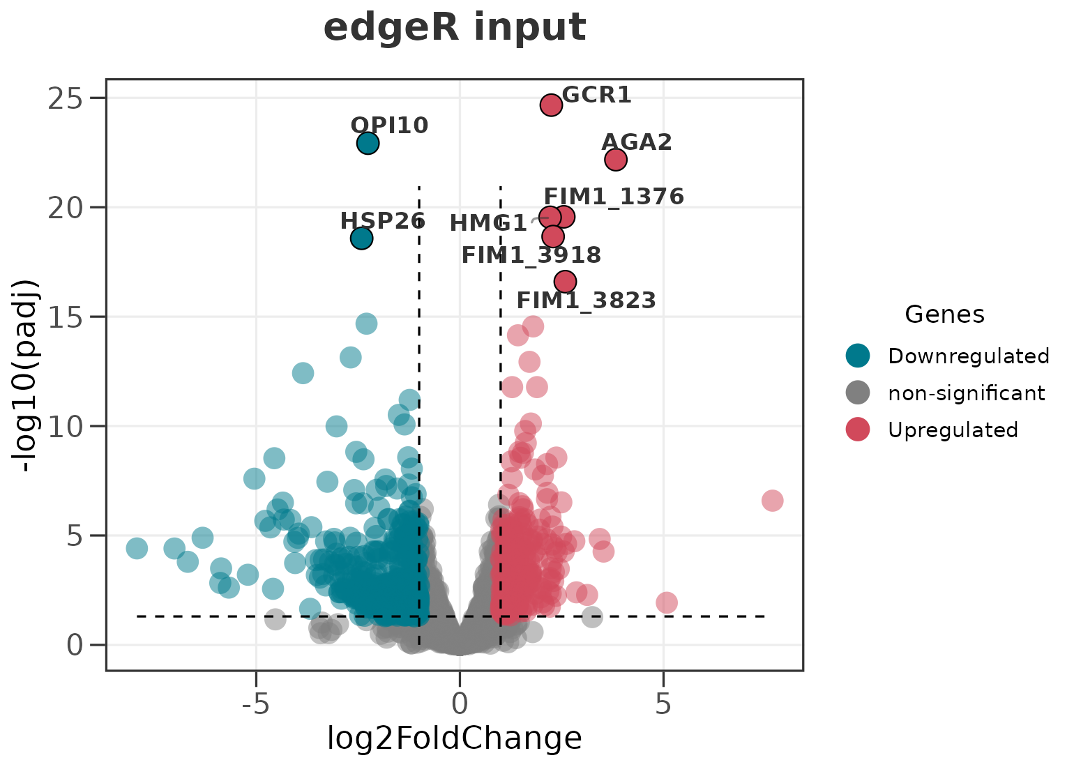

Pipeline	Fold change	p-value	adjusted p	expression
DESeq2 (`results()`)	`log2FoldChange`	`pvalue`	`padj`	`baseMean`
edgeR (`topTags()`)	`logFC`	`PValue`	`FDR`	`logCPM`
limma (`topTable()`)	`logFC`	`P.Value`	`adj.P.Val`	`AveExpr`

An interactive volcano

With the optional ggiraph package installed, interactive = TRUE returns a widget where hovering a point reveals the gene name and its statistics.

ggvolc(all_genes, attention_genes, interactive = TRUE)